Surface model (Water Overlay)

The Water Module's primary function is the simulation of the 2-dimensional flow of water on the surface. In order to simulate flowing water, the project area is discretized into x by y cells, based on the configured grid cell size.

Secondly a model is required which describes the rules that need to be followed. For this we use the two-dimensional Saint-Venant system, which reads:

In the Tygron Platform this model is implemented using the Well Balanced Positivity Preserving Central-Upwind Scheme described in Kurganov and Petrova (2007). For more information about the implementation, see Surface flow formula.

B = surface elevation of grid cell
h = water height of grid cell
w = water level of grid cell.

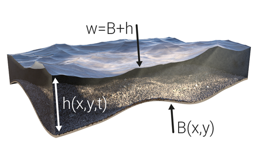
The implemented method rewrites the h from the original Saint-Venant system to w = h + z. See the image on the right for clarification on the terms water level, surface (or bottom) elevation and water height.

Flowing water

Based on variations in the surface elevation and water levels, which may cause unbalance, water will start flowing, until it eventually is balanced in terms of water level and fluxes hu and hv.

Water level initialization

In theory, each grid cell can have a unique water level and accompanying water height. In practice though, water levels are often initialized for large groups of cells, since it is assumed that a particular area within the project area has a given water level. Therefore, the surface water level is initialized based on hydrological features. We make the following distinction:

• Water levels of water terrains;
• Potential water levels for inundated land.

For all water terrains, the amount of water set on the grid cell is such that the resulting water level in that location is equal to the WATER_LEVEL attribute provided by the Water level area. If no water level area is overlapping that grid cell, or the water level is below the surface elevation of the grid cell, the water height is assumed to be 0 and the water level equal to the surface elevation.

For the second case, Inundation areas have been added to the model. Water is placed in all grid cells which are covered by an inundated area, (regardless of the terrain type in that location, in contrast to the water level areas), such that the resulting water level is again equal to the inundation area's INUNDATION_LEVEL attribute. If no inundation area is overlapping that grid cell, or the water level is below the surface elevation of the grid cell, the water height is assumed to be 0 and the water level equal to the surface elevation.

Notes

• Water can be added to and removed from the described surface system by Rain, Evaporation, Infiltration, certain Hydraulic structures and Breaches.
• Underground flow uses a different flow system and formula's, described in Underground model.
• In addition to water flowing between adjacent grid cells, water can also flow through hydraulic constructions. This is described in Hydraulic structures.

References

- ↑ Kurganov A, Petrova G (2007) ∙ A Second-Order Well-Balanced Positivity Preserving Central-Upwind Scheme for the Saint-Venant System ∙ found at: http://www.math.tamu.edu/~gpetrova/KPSV.pdf (last visited 2018-06-29)