Bottom flow pankow benchmark (Water Module): Difference between revisions
No edit summary |
|||
| (43 intermediate revisions by 2 users not shown) | |||
| Line 1: | Line 1: | ||
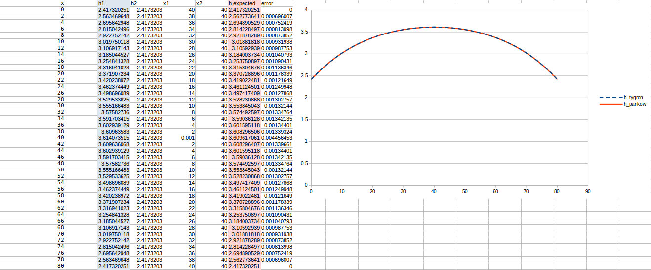
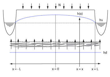
This | This [[Water Module benchmarks|benchmark]] demonstrates a situation where a parcel of land is situated between two waterways with a stable water level. In combination with [[Ground bottom flow formula (Water_Overlay)|ground water flowing from deeper ground layers through the bottom boundary]], a characteristic curve will form over time, as shown in the image below. It is described in a water balance research in 1968 of Pankow and Rijtema <ref name="Pankow68"/>, and also contains the accompanying formulas that describe the curve. | ||
In this case, we use the case which does not take into account the additional water flow resistance of the waterway. Secondly, rain could also be taken into account, but we set that to 0 to exclusively benchmark the | In this case, we use the case which does not take into account the additional water flow resistance of the waterway. Secondly, rain could also be taken into account, but we set that to 0 to exclusively benchmark the bottom flow mechanics. The continuous rainfall case is already tested in [[Freatic_groundwater_levels_benchmark_(Water_Module)|freatic groundwater levels benchmark]]. | ||
[[File:pankow_situation_benchmark.gif|A parcel of land situated between two waterways with | [[File:pankow_situation_benchmark.gif|frame|left|A parcel of land situated between two waterways with ground bottom flow and optional continuous rainfall<ref name="pankow"/>]] | ||
<br style="clear: both;"> | |||
===Formulas=== | ===Formulas=== | ||
Due to | Due to ground bottom flow and two stable water levels left and right, a specific ground water table curve will form. Part of the water flowed in from the bottom will flow left and part of the it will flow right. | ||
Note that the time at which this balance occurs is dependent on the starting situation. | Note that the time at which this balance occurs is dependent on the starting situation. | ||
| Line 20: | Line 21: | ||
Simplified without rain N: | Simplified without rain N: | ||
<math>h_d- | <math>h_1 = h_d - \frac{(h_1-h_2) cosh \frac{x_1}{\sqrt{KD \cdot c}}}{( cosh (\frac{x_2}{\sqrt{KD \cdot c} | ||
}) -1) - ( cosh (\frac{x_1}{\sqrt{KD \cdot c}}) -1) } </math> | }) -1) - ( cosh (\frac{x_1}{\sqrt{KD \cdot c}}) -1) } </math> | ||
To test the correctness of the | To test the correctness of the ground bottom flow, the formula can test the following condition with the accepted error margin <math>\epsilon</math>: | ||
<math>\frac{(h_1-h_2) cosh \frac{x_1}{\sqrt{KD \cdot c}}}{( cosh (\frac{x_2}{\sqrt{KD \cdot c} | |||
}) -1) - ( cosh (\frac{x_1}{\sqrt{KD \cdot c}}) -1) } | <math>\left | h_d - \frac{(h_1-h_2) cosh \frac{x_1}{\sqrt{KD \cdot c}}}{( cosh (\frac{x_2}{\sqrt{KD \cdot c} | ||
}) -1) - ( cosh (\frac{x_1}{\sqrt{KD \cdot c}}) -1) } - h_1 \right |< \epsilon</math> | |||
where: | where: | ||
: <math>x_1</math>: distance (m) of the point of measurement compared to the middle of the parcel. | : <math>x_1</math>: distance (m) of the point of measurement compared to the middle of the parcel. | ||
: <math>x_2</math>: distance (m) of the second point of measurement, which is always situated 3 meters from the edge of the waterway. | : <math>x_2</math>: distance (m) of the second point of measurement, which is always situated 3 meters from the edge of the waterway. | ||
: <math>h_1</math>: measured ground water level (m) at x_1 | : <math>h_1</math>: measured ground water level (m) at <math>x_1</math> | ||
: <math>h_2</math>: measured ground water level (m) at | : <math>h_2</math>: measured ground water level (m) at <math>x_2</math> | ||
: <math>h_d</math>: bottom head pressure | |||
: <math> | : <math>KD</math>: measured horizontal transmissivity of the ground layer (m2/day) | ||
: <math> | : <math>N</math>: additional ground water due to rainfall (m/day). | ||
: <math>N</math>: additional ground water (m/day). | |||
: <math>\epsilon</math>: accepted error margin | : <math>\epsilon</math>: accepted error margin | ||
===Setup=== | ===Setup=== | ||
The following setup | We use the following setup. The grid size used is 53 by 5, with a configurable cell size of <math>dx</math> in meters. There are two waterways, left and right, both with a stable water level of 3 meters. | ||
One inlet is placed on the cells x = 1 and y = 1 to 3 and an other is placed on the cells x = 52 and y - 1 to 3, with the following setup to ensure a stable water level: | |||
:[[Inlet_upper_threshold_(Water_Overlay)|UPPER_THRESHOLD]] set to 3 m. | |||
:[[Inlet_lower_threshold_(Water_Overlay)|LOWER_THRESHOLD]] set to 3 m. | |||
:[[Inlet q (Water Overlay)|Inlet Q]] set to 0, such that is unlimited. | |||
The terrain height is set to: | |||
<math>\begin {cases} | |||
0, & \text{if }x < 4 \text{ or } x > 48\\ | |||
1.5, & \text{if }x = 4 \text{ or } x = 48\\ | |||
3.5, & \text{if }x = 5 \text{ or } x = 47\\ | |||
5, & \text{otherwise} | |||
\end{cases}</math> | |||
Depending on the specific test case, the [[Bottom pressure prequel (Water Overlay)|Bottom head pressure]] <math>h_p</math> is set to: | |||
<math>\begin {cases} | |||
h_p, & \text{if }x > 5 \text{ and } x < 47\\ | |||
none, & \text{otherwise} | |||
\end{cases}</math> | |||
Similarly, the [[Bottom resistance prequel (Water Overlay)|Bottom resistance]] (in days) is set to: | |||
<math>\begin {cases} | |||
c, & \text{if }x > 5 \text{ and } x < 47\\ | |||
none, & \text{otherwise} | |||
\end{cases}</math> | |||
An aquifer can be added to configure the [[Aquifer kd (Water Overlay)|horizontal infiltration speed]]. An important thing to note here, is that the KD value used in the report <ref name="Pankow68"/> is derived from changes in water head over time, and does not mention the storage capacity of the soil. Therefor, in order to configure the Aquifer KD value in the {{software}}, the KD value has to be multiplied with the storage percentage. | |||
The [[Water level (Water Overlay)|water level]] is configured to 3 m for all cells, resulting in an initial water level above and below ground of 3 meters. | |||
The simulation time is set to n days, with | The simulation time is set to n days, with rain set to 0 mm. To configure this, the [[Weather rain m (Water Overlay)|rain]] set is set to <math>[3600 \cdot 24 \cdot n,0]</math>. | ||
===Results=== | ===Results=== | ||
==== | ====Test case 1==== | ||
:cell size: 10 m; | |||
[[File: | :<math>KD</math>: 17 m²/day; | ||
:Water storage fraction: 0.10; | |||
:Aquifer KD configured to 1.7 m²/day in the {{software}}; | |||
:Bottom resistance <math>c</math>: 20 days | |||
:Bottom head pressure <math>h_d</math>: 4.1 | |||
:Simulation days <math>n</math>: 128 days | |||
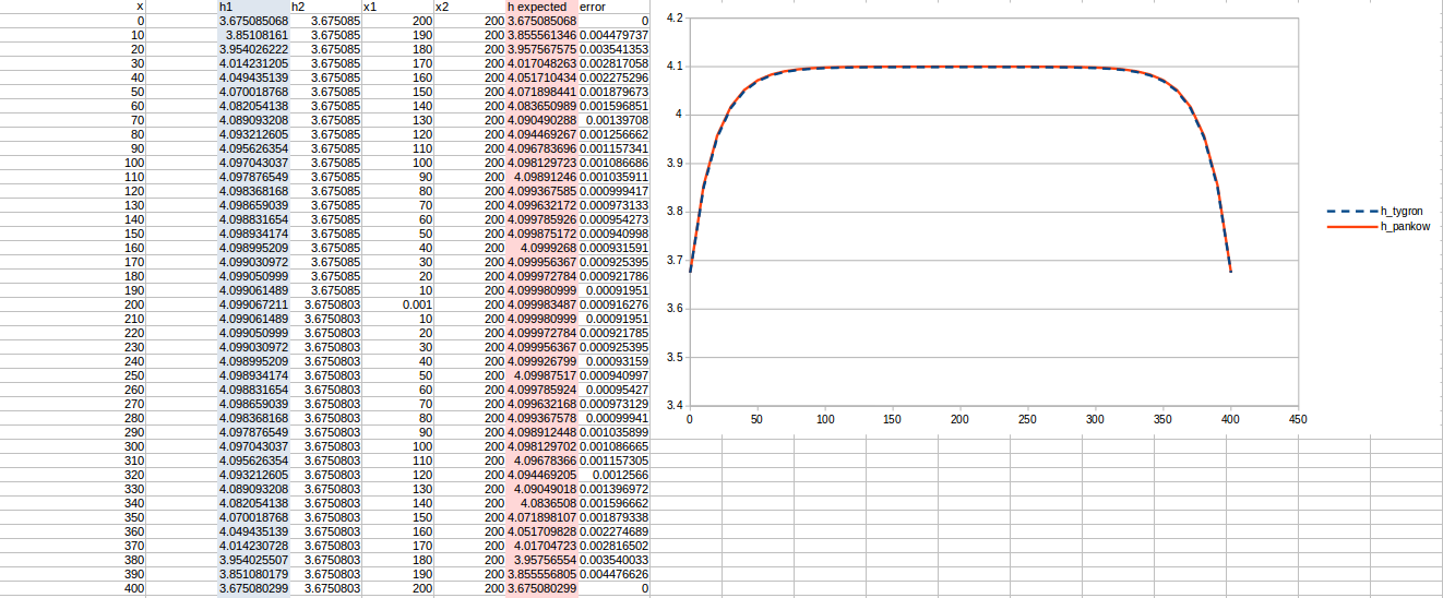
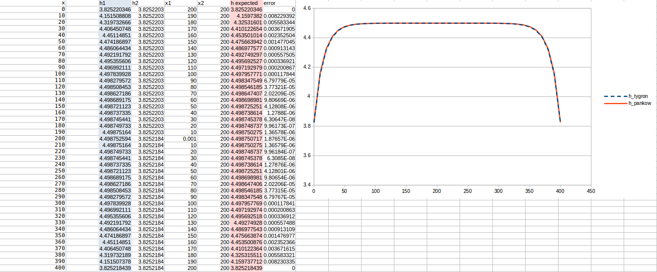
[[File:128days_10m_kd17_c20_ws10_h4_1.png]] | |||
====Test case 2==== | |||
:cell size: 10 m; | |||
:<math>KD</math>: 22 m²/day; | |||
:Water storage fraction: 0.25; | |||
:Aquifer KD configured to 5.5 m²/day in the {{software}}; | |||
:Bottom resistance <math>c</math>: 40 days | |||
:Bottom head pressure <math>h_d</math>: 4.1 | |||
:Simulation days <math>n</math>: 128 days | |||
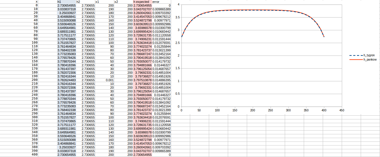
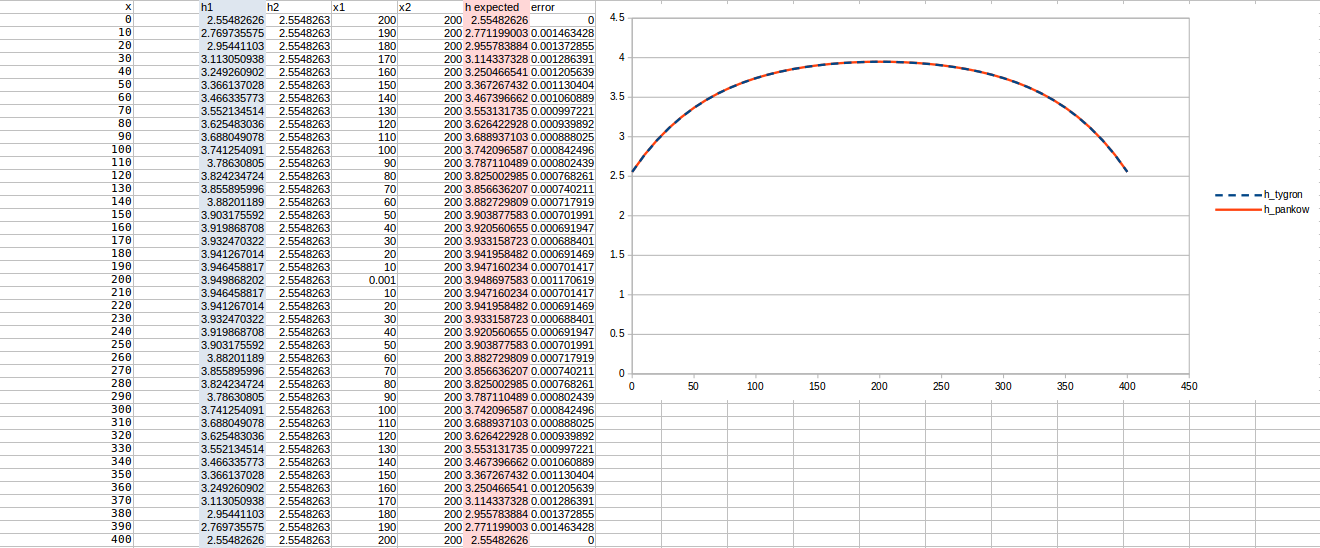
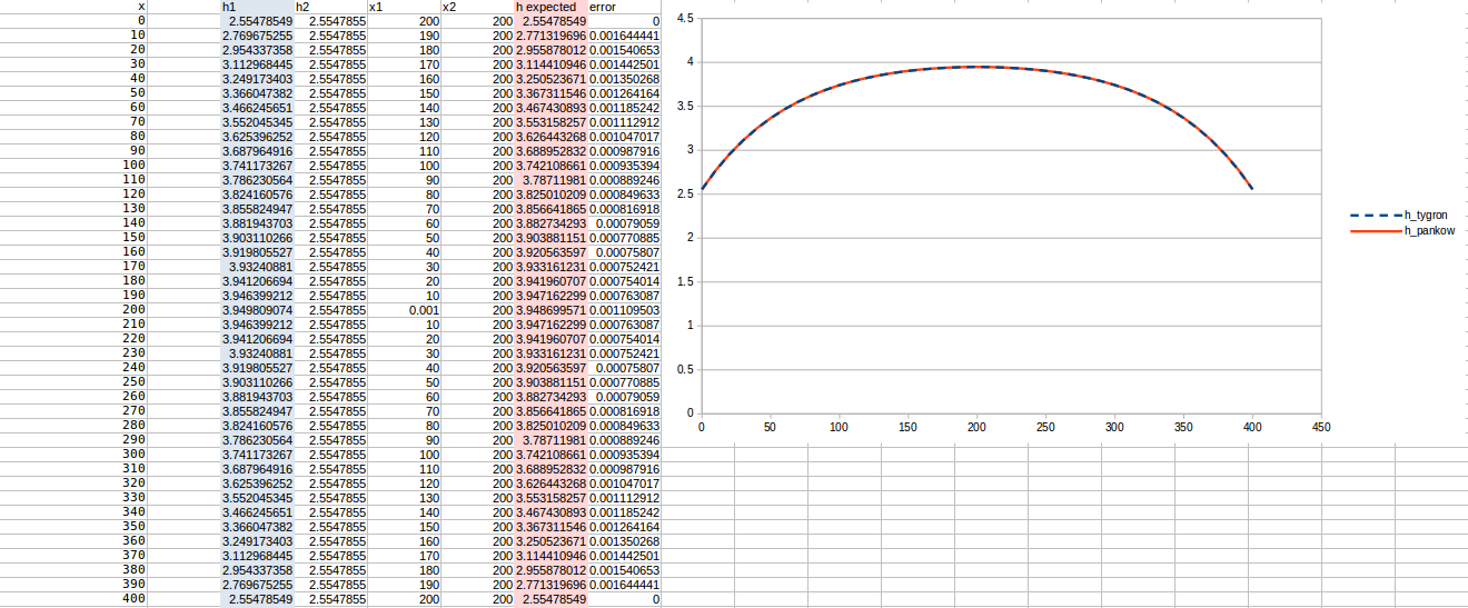
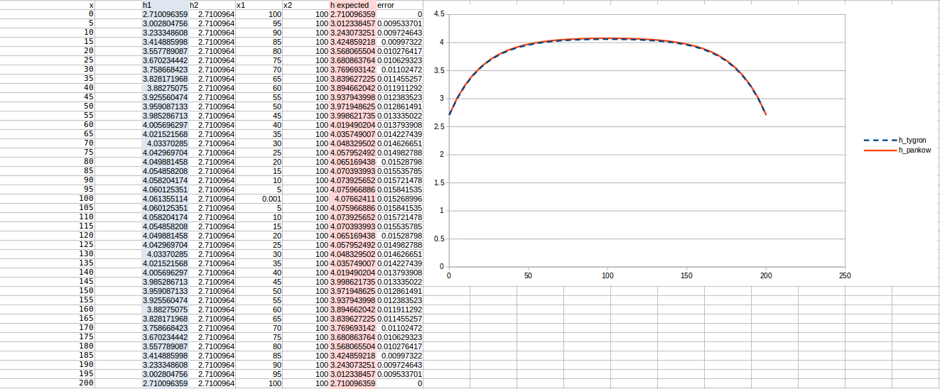
[[File:128days_10m_kd22_c40_ws25_h4_1.png]] | |||
====Test case 3==== | |||
:cell size: 10 m; | |||
:<math>KD</math>: 22 m²/day; | |||
:Water storage fraction: 0.25; | |||
:Aquifer KD configured to 5.5 m²/day in the {{software}}; | |||
:Bottom resistance <math>c</math>: 40 days | |||
:Bottom head pressure <math>h_d</math>: 3.8 | |||
:Simulation days <math>n</math>: 128 days | |||
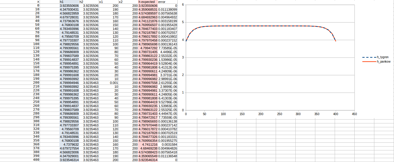
[[File:128days_10m_kd22_c40_ws25_h3_8.png]] | |||
====Test case 4==== | |||
:cell size: 10 m; | |||
:<math>KD</math>: 22 m²/day; | |||
:Water storage fraction: 0.25; | |||
:Aquifer KD configured to 5.5 m²/day in the {{software}}; | |||
:Bottom resistance <math>c</math>: 10 days | |||
:Bottom head pressure <math>h_d</math>: 4.8 | |||
:Simulation days <math>n</math>: 128 days | |||
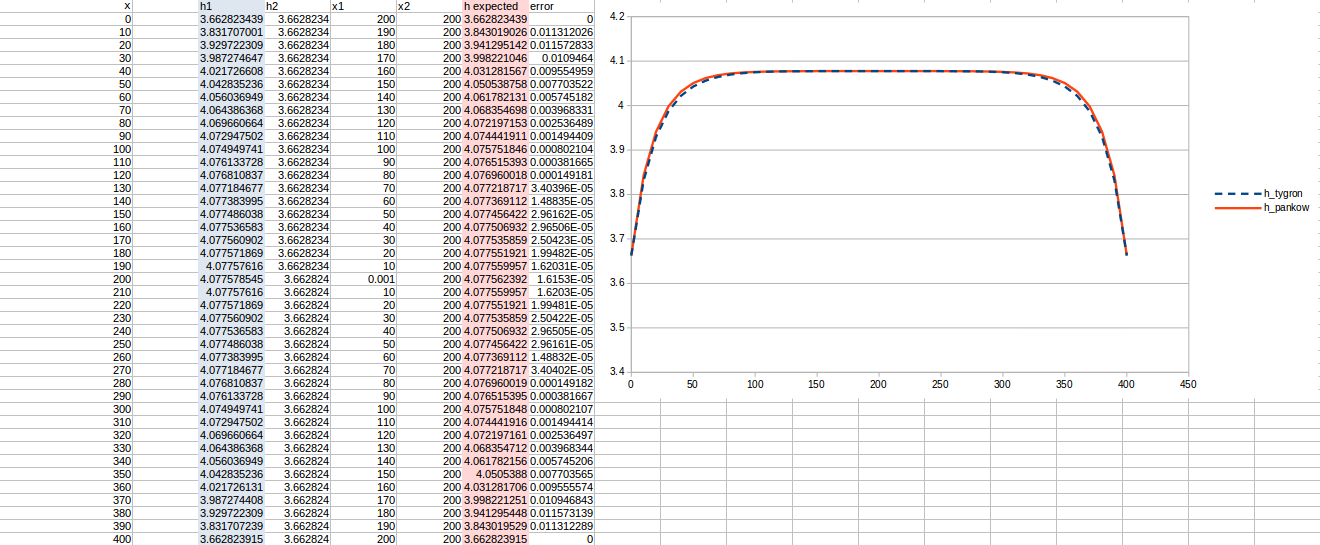
[[File:128days_10m_kd22_c10_ws25_h4_8.png]] | |||
====Test case 5==== | |||
:cell size: 10 m; | |||
:<math>KD</math>: 17 m²/day; | |||
:Water storage fraction: 0.10; | |||
:Aquifer KD configured to 1.7 m²/day in the {{software}}; | |||
:Bottom resistance <math>c</math>: 20 days | |||
:Bottom head pressure <math>h_d</math>: 4.1 (but leads to <math>h_d=4.077</math> for the comparisons with the middle value) | |||
:Simulation days <math>n</math>: 64 days | |||
[[File:64days_10m_kd17_c20_ws10_h4_1.png]] | |||
====Test case 6==== | |||
:cell size: 10 m; | |||
:<math>KD</math>: 22 m²/day; | |||
:Water storage fraction: 0.33; | |||
:Aquifer KD configured to 7.26 m²/day in the {{software}}; | |||
:Bottom resistance <math>c</math>: 10 days | |||
:Bottom head pressure <math>h_d</math>: 4.5 (but leads to <math>h_d=4.499</math> for the comparisons with the middle value) | |||
:Simulation days <math>n</math>: 64 days | |||
[[File:64days_10m_kd22_c10_ws33_h4_5.png]] | |||
====Test case 7==== | |||
:cell size: 10 m; | |||
:<math>KD</math>: 220 m²/day; | |||
:Water storage fraction: 0.25; | |||
:Aquifer KD configured to 55 m²/day in the {{software}}; | |||
:Bottom resistance <math>c</math>: 20 days | |||
:Bottom head pressure <math>h_d</math>: 4.1 | |||
:Simulation days <math>n</math>: 64 days | |||
[[File:64days_10m_kd220_c20_ws25_h4_1.png]] | |||
====Test case 8==== | |||
:cell size: 10 m; | |||
:<math>KD</math>: 220 m²/day; | |||
:Water storage fraction: 0.10; | |||
:Aquifer KD configured to 55 m²/day in the {{software}}; | |||
:Bottom resistance <math>c</math>: 20 days | |||
:Bottom head pressure <math>h_d</math>: 4.1 | |||
:Simulation days <math>n</math>: 64 days | |||
[[File:64days_10m_kd220_c20_ws10_h4_1.png]] | |||
====Test case 9==== | |||
:cell size: 5 m; | |||
:<math>KD</math>: 22 m²/day; | |||
:Water storage fraction: 0.10; | |||
:Aquifer KD configured to 2.2 m²/day in the {{software}}; | |||
:Bottom resistance <math>c</math>: 20 days | |||
:Bottom head pressure <math>h_d</math>: 4.1 | |||
:Simulation days <math>n</math>: 64 days | |||
[[File:64days_5m_kd22_c20_ws10_h4_1.png]] | |||
==== | ====Test case 10==== | ||
:cell size: 2 m; | |||
[[File: | :<math>KD</math>: 22 m²/day; | ||
:Water storage fraction: 0.10; | |||
:Aquifer KD configured to 2.2 m²/day in the {{software}}; | |||
:Bottom resistance <math>c</math>: 20 days | |||
:Bottom head pressure <math>h_d</math>: 4.1 | |||
:Simulation days <math>n</math>: 64 days | |||
[[File:64days_2m_kd22_c20_ws10_h4_1.png]] | |||
===Notes=== | ===Notes=== | ||
* | * A higher KD value can lead to a lower stable ground water level than the [[Bottom pressure prequel (Water Overlay)|head pressure]]. | ||
===References=== | ===References=== | ||
<references> | <references> | ||
<ref name=" | <ref name="Pankow68">J. Pankow en P.E. Rijtema, 1970. De resultaten van het waterbalansonderzoek in 1968 voor de objecten met een constant slootpeil in Hoenkoop. Nota 567. Instituut voor Cultuurtechniek en Waterhuishouding, Wageningen.</ref> | ||
<ref name="pankow">Schatten van kwel (Pankow), Grondwaterformules.nl/index.php/formules/ontwatering/kwel-berekenen-pankow</ref> | |||
</references> | </references> | ||
{{Water Module buttons}} | {{Water Module buttons}} | ||
Latest revision as of 14:50, 5 March 2024
This benchmark demonstrates a situation where a parcel of land is situated between two waterways with a stable water level. In combination with ground water flowing from deeper ground layers through the bottom boundary, a characteristic curve will form over time, as shown in the image below. It is described in a water balance research in 1968 of Pankow and Rijtema [1], and also contains the accompanying formulas that describe the curve. In this case, we use the case which does not take into account the additional water flow resistance of the waterway. Secondly, rain could also be taken into account, but we set that to 0 to exclusively benchmark the bottom flow mechanics. The continuous rainfall case is already tested in freatic groundwater levels benchmark.
Formulas
Due to ground bottom flow and two stable water levels left and right, a specific ground water table curve will form. Part of the water flowed in from the bottom will flow left and part of the it will flow right. Note that the time at which this balance occurs is dependent on the starting situation.
The following formula, taken from [1], describes the curve of ground water levels when the ground water flow to the left and right have become stable:
Simplified without rain N:
To test the correctness of the ground bottom flow, the formula can test the following condition with the accepted error margin :
where:
- : distance (m) of the point of measurement compared to the middle of the parcel.
- : distance (m) of the second point of measurement, which is always situated 3 meters from the edge of the waterway.
- : measured ground water level (m) at
- : measured ground water level (m) at
- : bottom head pressure
- : measured horizontal transmissivity of the ground layer (m2/day)
- : additional ground water due to rainfall (m/day).
- : accepted error margin
Setup
We use the following setup. The grid size used is 53 by 5, with a configurable cell size of in meters. There are two waterways, left and right, both with a stable water level of 3 meters.
One inlet is placed on the cells x = 1 and y = 1 to 3 and an other is placed on the cells x = 52 and y - 1 to 3, with the following setup to ensure a stable water level:
- UPPER_THRESHOLD set to 3 m.
- LOWER_THRESHOLD set to 3 m.
- Inlet Q set to 0, such that is unlimited.
The terrain height is set to:
Depending on the specific test case, the Bottom head pressure is set to:
Similarly, the Bottom resistance (in days) is set to:
An aquifer can be added to configure the horizontal infiltration speed. An important thing to note here, is that the KD value used in the report [1] is derived from changes in water head over time, and does not mention the storage capacity of the soil. Therefor, in order to configure the Aquifer KD value in the Tygron Platform, the KD value has to be multiplied with the storage percentage.
The water level is configured to 3 m for all cells, resulting in an initial water level above and below ground of 3 meters.
The simulation time is set to n days, with rain set to 0 mm. To configure this, the rain set is set to .
Results
Test case 1
- cell size: 10 m;
- : 17 m²/day;
- Water storage fraction: 0.10;
- Aquifer KD configured to 1.7 m²/day in the Tygron Platform;
- Bottom resistance : 20 days
- Bottom head pressure : 4.1
- Simulation days : 128 days
Test case 2
- cell size: 10 m;
- : 22 m²/day;
- Water storage fraction: 0.25;
- Aquifer KD configured to 5.5 m²/day in the Tygron Platform;
- Bottom resistance : 40 days
- Bottom head pressure : 4.1
- Simulation days : 128 days
Test case 3
- cell size: 10 m;
- : 22 m²/day;
- Water storage fraction: 0.25;
- Aquifer KD configured to 5.5 m²/day in the Tygron Platform;
- Bottom resistance : 40 days
- Bottom head pressure : 3.8
- Simulation days : 128 days
Test case 4
- cell size: 10 m;
- : 22 m²/day;
- Water storage fraction: 0.25;
- Aquifer KD configured to 5.5 m²/day in the Tygron Platform;
- Bottom resistance : 10 days
- Bottom head pressure : 4.8
- Simulation days : 128 days
Test case 5
- cell size: 10 m;
- : 17 m²/day;
- Water storage fraction: 0.10;
- Aquifer KD configured to 1.7 m²/day in the Tygron Platform;
- Bottom resistance : 20 days
- Bottom head pressure : 4.1 (but leads to for the comparisons with the middle value)
- Simulation days : 64 days
Test case 6
- cell size: 10 m;
- : 22 m²/day;
- Water storage fraction: 0.33;
- Aquifer KD configured to 7.26 m²/day in the Tygron Platform;
- Bottom resistance : 10 days
- Bottom head pressure : 4.5 (but leads to for the comparisons with the middle value)
- Simulation days : 64 days
Test case 7
- cell size: 10 m;
- : 220 m²/day;
- Water storage fraction: 0.25;
- Aquifer KD configured to 55 m²/day in the Tygron Platform;
- Bottom resistance : 20 days
- Bottom head pressure : 4.1
- Simulation days : 64 days
Test case 8
- cell size: 10 m;
- : 220 m²/day;
- Water storage fraction: 0.10;
- Aquifer KD configured to 55 m²/day in the Tygron Platform;
- Bottom resistance : 20 days
- Bottom head pressure : 4.1
- Simulation days : 64 days
Test case 9
- cell size: 5 m;
- : 22 m²/day;
- Water storage fraction: 0.10;
- Aquifer KD configured to 2.2 m²/day in the Tygron Platform;
- Bottom resistance : 20 days
- Bottom head pressure : 4.1
- Simulation days : 64 days
Test case 10
- cell size: 2 m;
- : 22 m²/day;
- Water storage fraction: 0.10;
- Aquifer KD configured to 2.2 m²/day in the Tygron Platform;
- Bottom resistance : 20 days
- Bottom head pressure : 4.1
- Simulation days : 64 days
Notes
- A higher KD value can lead to a lower stable ground water level than the head pressure.
References
- ↑ 1.0 1.1 1.2 J. Pankow en P.E. Rijtema, 1970. De resultaten van het waterbalansonderzoek in 1968 voor de objecten met een constant slootpeil in Hoenkoop. Nota 567. Instituut voor Cultuurtechniek en Waterhuishouding, Wageningen.
- ↑ Schatten van kwel (Pankow), Grondwaterformules.nl/index.php/formules/ontwatering/kwel-berekenen-pankow


![{\displaystyle [3600\cdot 24\cdot n,0]}](https://wikimedia.org/api/rest_v1/media/math/render/svg/16f6d65e7c78515851224e0a56b09a84625ef3ce)


