Bottom flow pankow benchmark (Water Module)

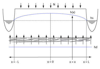
This testcase demonstrates a situation where a parcel of land is situated between two waterways with a stable water level. In combination with seepage, a characteristic curve will form over time, as shown in the image below. It is described in a water balance research in 1968 of Pankow and Rijtema , and also contain the accompanying formulas that describe the curve. In this case, we use the case which does not take into account the additional water flow resistance of the waterway. Secondly, rain could also be taken into account, but we set that to 0 to exclusively benchmark the seepage mechanics. The continuous rainfall case is already tested in freatic groundwater levels benchmark.

Formulas

Due to seepage and two stable water levels left and right, a specific ground water table curve will form. Part of the water seeped in will flow left and part of the it will flow right. Note that the time at which this balance occurs is dependent on the starting situation.

The following formula, taken from , describes the curve of ground water levels when the ground water flow to the left and right have become stable:

$A={\frac {(h_{1}-h_{2})cosh{\frac {x_{1}}{\sqrt {KD\cdot c}}}}{{\frac {x_{2}^{2}}{2KD}}\cdot {\frac {2KD\cdot c}{x_{2}^{2}}}\cdot (cosh({\frac {x_{2}}{\sqrt {KD\cdot c}}})-1)-{\frac {x_{1}^{2}}{2KD}}\cdot {\frac {2KD\cdot c}{x_{1}^{2}}}\cdot (cosh({\frac {x_{1}}{\sqrt {KD\cdot c}}})-1)}}={\frac {(h_{1}-h_{2})cosh{\frac {x_{1}}{\sqrt {KD\cdot c}}}}{c\cdot (cosh({\frac {x_{2}}{\sqrt {KD\cdot c}}})-1)-c\cdot (cosh({\frac {x_{1}}{\sqrt {KD\cdot c}}})-1)}}$

$A=N+{\frac {h_{d}-h_{1}}{c}}$

Simplified without rain N:

Failed to parse (MathML with SVG or PNG fallback (recommended for modern browsers and accessibility tools): Invalid response ("Math extension cannot connect to Restbase.") from server "https://wikimedia.org/api/rest_v1/":): {\displaystyle \frac{h_d-h_1}{c} = \frac{(h_1-h_2) cosh \frac{x_1}{\sqrt{KD \cdot c}}}{c \cdot ( cosh (\frac{x_2}{\sqrt{KD \cdot c} }) -1) - c \cdot ( cosh (\frac{x_1}{\sqrt{KD \cdot c} where: : <math>x_1} : distance (m) of the point of measurement compared to the middle of the parcel.

$x_{2}$: distance (m) of the second point of measurement, which is always situated 3 meters from the edge of the waterway.

$h_{1}$: measured ground water level (m) at x_1

$h_{2}$: measured ground water level (m) at x_2

$h_{d}$: seepage head

$KD$: distance between both waterways (m)

$k$: horizontal infiltration speed (m / day)

$N$: additional ground water (m/day).

Setup

The following setup has been taken from the use case Peilverschil over een strook grond (freatisch) at grondwaterformules.nl.

In the situation described there, the chosen Length L is set to 500 m. This is achieved with a grid size of 28 by 5, with a cell size of 20 m. There are two stable ground water levels, one on left of 11 meters (datum) and one on the right at 10 meters (datum). The rainfall is 0.8 mm per day, the horizontal infiltration speed is 3 m per day.

The terrain height is set to 12 for all cells and the ground bottom distance is also set to 12.

The terrain type's infiltration speed can be configured to 3 m / day.

For x = 1 the initial ground water level is set to 11 and for x = 26 the ground water level is set to 10. The initial ground water levels between this points is linearly interpolated.

Additionally, two underground inlets are placed, one on x=1 and one on x=26, as an area over y = 1 to 3.

The simulation time is set to n days, with a rainfall of 0.8 mm per day. To configure this, the rain set is set to $[3600\cdot 24\cdot n,{\frac {0.8}{1000\cdot 3600\cdot 24}}]$.

Results

365 days

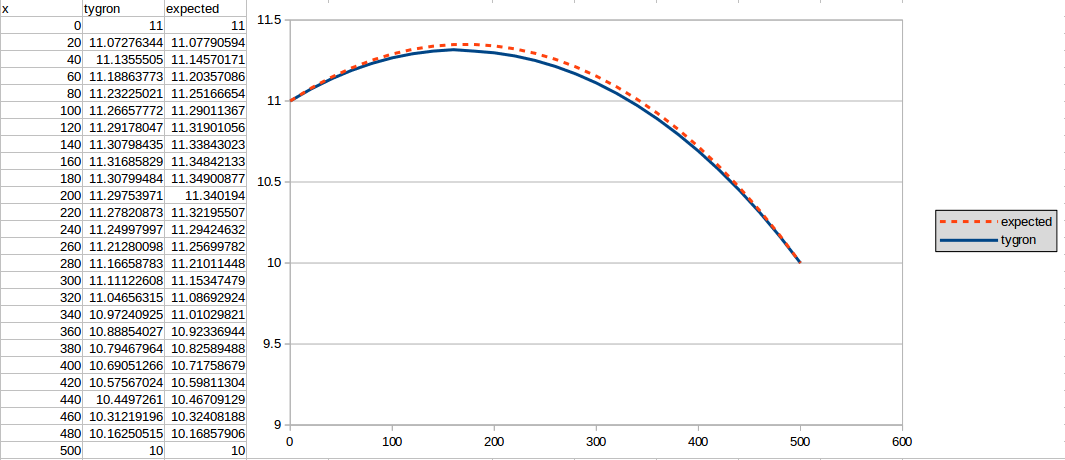
The first result is generated for n = 365:

730 days

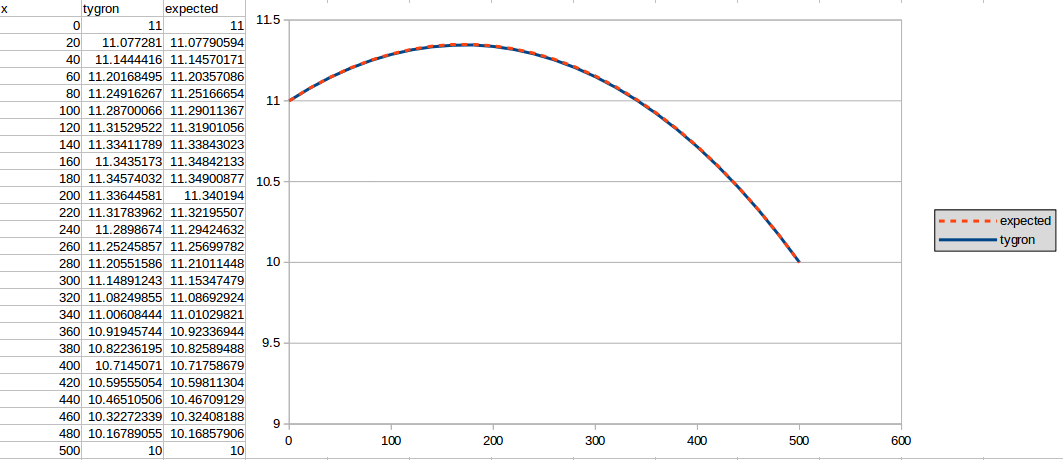
The second result is generated using n = 730:

Notes

• The amount of days it takes to reach the stable solution is highly dependent on the starting situation.

References

Water Module

Tutorials

Overview

Theory

Benchmarks