Testbed tutorial: Difference between revisions
No edit summary |
|||
| (131 intermediate revisions by 3 users not shown) | |||
| Line 1: | Line 1: | ||
{{tutorial prerequisites | {{tutorial prerequisites | ||
|tutorial=This tutorial relies on base knowledge about the editor interface. | |tutorial=This tutorial relies on base knowledge about the editor interface. | ||
|project=This tutorial can be followed in an empty project area. | |project=This tutorial can be followed in an empty project area. | ||
|required-excel= | |required-excel= | ||
|additional= | |additional=Knowledge of the functioning of the water module is recommended, but not required. | ||
|Create a new, empty project, sized to 500m by 500m. Ensure the unit system is set to "International". Also ensure it's an empty project area, not based on a real world location. | |Create a new, empty project, sized to 500m by 500m. Ensure the unit system is set to "International". Also ensure it's an empty project area, not based on a real world location. | ||
}} | }} | ||
| Line 13: | Line 12: | ||
In the {{software}}, whenever you create a project based on real-world data, the project is populated with a wide range of data. Virtually every project area contains numerous constructions, height differentials, and terrain types. If any calculation takes place, especially spatial calculations, all that data can serve as input. That makes it a lot more difficult to see exactly how a specific element factors into a specific result, or where the difference between an expected and actual result comes from. | In the {{software}}, whenever you create a project based on real-world data, the project is populated with a wide range of data. Virtually every project area contains numerous constructions, height differentials, and terrain types. If any calculation takes place, especially spatial calculations, all that data can serve as input. That makes it a lot more difficult to see exactly how a specific element factors into a specific result, or where the difference between an expected and actual result comes from. | ||
For this reason, what characterizes a testbed most is the absence of data. Anything that is not | Testbeds can serve the following purposes: | ||
* Quick investigations into how a specific functionality works | |||
* Demonstrations of multiple functionalities | |||
* Forming a baseline for consistency testing | |||
* Testing for (and demonstrations of) bugs or other issues | |||
For this reason, what characterizes a testbed most is the absence of data. Anything that is not required for a specific case is left out, or at least left in a uniform, invariable state. | |||
{{page_break}} | |||
===Starting point=== | ===Starting point=== | ||
| Line 22: | Line 28: | ||
* There is a uniform height map, with the height of the terrain set to 1m relative to {{datum}}. | * There is a uniform height map, with the height of the terrain set to 1m relative to {{datum}}. | ||
* The surface of the terrain is | * The surface of the terrain is the "Open Land" type. The underground terrain is the "Unknown" type. | ||
* There is only a single municipal stakeholder, as a stakeholder to select for an editing user. The entirety of the | * There is only a single municipal stakeholder, as a stakeholder to select for an editing user. The entirety of the [[project area]] is owned by that stakeholder. | ||
* There are 4 neighborhoods (north-west, north-east, south-west, south-east), or if the project area is small, 1 single neighborhood. | * There are 4 neighborhoods (north-west, north-east, south-west, south-east), or if the project area is small, 1 single neighborhood. | ||
* There is no zoning plan. | * There is no zoning plan. | ||
* There are no construction. | * There are no construction. | ||
* The upper-left spatial coordinates of the project area are set to 0 degrees latitude and longitude. | * The upper-left spatial coordinates of the project area are set to 0 degrees latitude and longitude. | ||
{{page_break}} | |||
== | ==Quick functionality testing== | ||
Testbeds can be used to test specific implementation questions. | Testbeds can be used to test specific implementation questions. The question you're going to investigate is how the average overlay calculation functions in cases where the calculation takes place near the edge of the project area. | ||
The average overlay functions, for any given grid cell, by looking at the surrounding grid cells, calculating the average value of the cells found. In most locations in a project area this calculation is very straightforward. However, if any of the cells looked at would fall outside the project area, any number of behaviors could be reasonable. For example: the cells outside the project area could be assumed to have a certain default value, or the cells could be disregarded for the calculations. You will configure the testbed to reveal how the average overlay deals with cells outside the project area. | |||
Start by adding the overlay we're going to test. Add an average overlay to the project. | Start by adding the overlay we're going to test. Add an [[Average Overlay|average overlay]] to the project. | ||
[[File:AddAverageOverlay.jpg|350px|frame|center|Add an average overlay.]] | [[File:AddAverageOverlay.jpg|350px|frame|center|Add an average overlay.]] | ||
{{page_break}} | |||
Prepare the overlay in such a way that it will calculate the spatial average of a user-defined attribute. As Filter Attribute, enter "AVGTEST". Also set the Cell averaging distance to 50m. This will ensure that multiple entities can be drawn in the map and be spatially calculated, without necessarily affecting each other's outcomes. | Prepare the overlay in such a way that it will calculate the spatial average of a user-defined attribute. As Filter Attribute, enter "AVGTEST" in the General tab in the right panel. Also set the Cell averaging distance to 50m. This will ensure that multiple entities can be drawn in the map and be spatially calculated, without necessarily affecting each other's outcomes. | ||
[[File:Testbed_AverageOverlaySettings.jpg|350px|frame|center|Configure the average overlay to calculate using a user-defined attribute, and a relatively small radius.]] | [[File:Testbed_AverageOverlaySettings.jpg|350px|frame|center|Configure the average overlay to calculate using a user-defined attribute, and a relatively small radius.]] | ||
With this configuration, the calculation will result in a value of 0 in every location. | With this configuration, the calculation will result in a value of 0 in every location. | ||
[[File:Testbed_AverageOverlayZero.jpg|350px|frame|center|In the first setup situation, the result of the average calculation is 0, everywhere.]] | [[File:Testbed_AverageOverlayZero.jpg|350px|frame|center|In the first setup situation, the result of the average calculation is 0, everywhere.]] | ||
{{page_break}} | |||
Now add a construction to the project, and place it more or less in the center of the project. Make sure you use the block-based brush, and draw in exactly 1 block (10m by 10m, for a total of 100m²). | Now add a construction to the project, and place it more or less in the center of the project. Make sure you use the block-based brush, and draw in exactly 1 block (10m by 10m, for a total of 100m²). | ||
[[File:Testbed_DrawConstruction.jpg|350px|frame|center|Draw a construction, with the size of a single 10m by 10m block.]] | [[File:Testbed_DrawConstruction.jpg|350px|frame|center|Draw a construction, with the size of a single 10m by 10m block.]] | ||
Add an AVGTEST attribute to the construction, with a value of 1000. | |||
[[File:Testbed_ConstructionAttribute.jpg|350px|frame|center|Assign an AVGTEST attribute with value 1000 to the construction.]] | |||
Switch back to the average overlay in the editor, and select "Update Now" to recalculate the content | |||
{{page_break}} | |||
Now, if you open the average overlay, you will see the construction is the center of a large area where the average value of AVGTEST is higher than in all other locations in the project area. | |||
[[File:Testbed_AvgConstruction1.jpg|350px|frame|center|The average value at the location of the construction is around 130.]] | |||
This setup creates a first look into how the average overlay functions. In the exact location of the construction, and its direct surroundings, the average value of AVGTEST is around 130. It tapers of at a distance of about 50 meters. | |||
''Note that you may see a value lower than 130, based on the exact location you have placed the construction. This is due to the construction's alignment on the calculation grid. This is expected, and does not affect the principles explained next. Take note of the value you see in your project, and continue.'' | |||
We can now add another construction to the project, again with an AVGTEST attribute set to a value of 1000, and place that construction in the corner of the project area. Again, making sure that the construction is exactly 1 block of 10m by 10m, for a total of 100m². | |||
Recalculating the overlay and looking at the average value at the location of the new construction gives an average value of 180. | |||
[[File:Testbed_AvgConstruction2.jpg|350px|frame|center|The average value at the location of the construction is around 180.]] | |||
The fact that the calculated value in the corner is higher indicates that the cells outside the project area don't have an assumed value of 0 or lower. | |||
{{page_break}} | |||
Increase the AVGTEST attribute value of both constructions to 2000, and check again what average values are calculated in the locations of the constructions. | |||
[[File:Testbed_ConstructionAttribute2.jpg|350px|frame|center|Change the value of the AVGTEST attribute to 2000, double what it was before.]] | |||
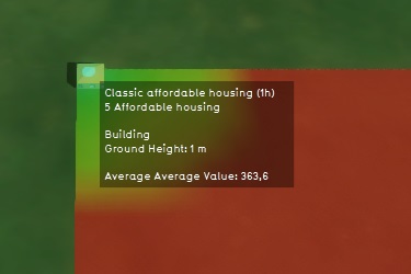
Now when you look at the calculated average value at the location of the construction, you will see that after doubling the attribute of the construction, the calculated value has doubled as well (give or take a rounding). | |||
[[File:Testbed_AvgConstruction3.jpg|350px|frame|center|The value calculated has doubled.]] | |||
{{page_break}} | |||
We can now put the following facts together: | |||
* An average is a value calculated as follows: The sum of all values found in the calculation area, divided by the calculation area. | |||
* The calculated average scales linearly with the value of the object we place. This means that the cells outside the project area do not have a positive or negative value. If they did, the impact of raising or lowering the attribute value would have been more or less impactful. | |||
* An object at the edge of the project area has a greater impact on the calculated spatial average than a construction in the middle of the project area. This means that either the sum of all values increases as we get closer to the edge, or the surface area we divide by decreases. | |||
We can determine that because the summed value does not change, the surface area used in the calculation must decrease in order to see the higher result. Thus our conclusion is that potential cells outside the project area are not used in the calculation of a spatial average. | |||
{{page_break}} | |||
===Considerations=== | |||
Note that based on the conclusion we have drawn, you may be tempted to expect the calculated values to match more neatly. Specifically, if the construction in the middle of the map has a full circle around it in which to perform its calculation, the construction in the edge of the map must have a quarter of the area of similar circle, thus the values should differ by a factor of 4. However, due to the layout of the constructions on the grid this is not the case. | |||
[[File:TestBed_ExampleGrid3.jpg|350px|frame|center|Schematic functioning of the grid for spatial averaging calculations. Left: the circle taken into consideration given a specific cell in the middle of the map. Right: the section of the circle taken into consideration when the specific cell is at the corner of the map. Notice the area of the section on the right is not an exact quarter of the section on the left.]] | |||
Also note that based on the exact size, placement, and rounding of values and polygons, it may be difficult to derive the outcomes seen from the base values without greater insight into the exact interpretations the {{software}} makes. This is to be expected, and the approach used here functions regardless of those exact calculations. | |||
{{page_break}} | |||
{{header|level=3|color=#c45911|Assignments}} | |||
These assignments are designed to demonstrate further means of experimentation. | |||
<ol> | |||
<li>Knowing the radius of the spatial calculation is 50m, place a construction with the same attribute and value as close to the edge of the map as possible without the calculated average value differing from the construction in the middle of the project area.</li> | |||
<li>Change the average attribute of the constructions back to 1000, and instead expand both constructions with another block of 10m by 10m. Both constructions should be exactly twice as large as they were.</li> | |||
<li>Knowing the grid cell size is exactly 10m by 10m, find an explanation for the fact that both 'sides' of the construction in the middle of the map have the same calculated average, but the sides of the construction in the corner of the map do not.</li> | |||
</ol> | |||
{{page_break}} | |||
==Calculation insights== | |||
Testbeds, due to their inherent simplicity, can in some cases also be used to retrace exact calculations. The question you're going to investigate now is the size of the inactive border of the flooding overlay's calculation. | |||
The calculation occurs in a grid, but the outer edge of grid cells is inactive. This means that there may be a discrepancy between input for the calculation and the results seen. If the exact number of cells can be determined, this discrepancy can be accounted for. | |||
Either create a new empty project with the same specifications as in the prerequisites, or clean up the project configured during the last assignment by removing the added overlay and construction. Either way, make sure you start with an empty project area again. | |||
Start by adding the overlay we are going to test. Add a flooding overlay to the project. | |||
[[File:AddFloodingOverlay.jpg|350px|frame|center|Add a flooding overlay to the project.]] | |||
{{page_break}} | |||
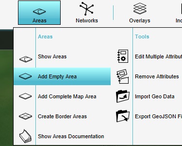
Add an area to the project, covering the complete project area. | |||
[[File:AddCompleteArea.jpg|350px|frame|center|Add an area for the complete map.]] | |||
Add an INUNDATION_LEVEL attribute to the area, set to a value of 2. | |||
[[File:Testbed_CompleteArea.jpg|350px|frame|center|Add an area for the complete map.]] | |||
This area will now cause the flooding overlay to initialize the calculation with a layer of 1 meter of water across the entire project area. (The project area's default height is 1 meter above {{datum}}, and the height of the water will be set to 2 meters above {{datum}}.) | |||
{{page_break}} | |||
Activate the flooding overlay, and notice the entire project area is colored blue, indicating the presence of water. Click anywhere in the project area to see a "Flooding" height of 1 meter is calculated. If needed please make sure to calculate the area and overlay with the recalculate button in the upper left corner. | |||
[[File:Testbed_CompleteWaterResult.jpg|350px|frame|center|Add an area for the complete map.]] | |||
Select the flooding overlay in the editor, and select the "Show Water Balance" option. | |||
[[File:Testbed_WaterBalance1.jpg|350px|frame|center|Open the water balance.]] | |||
{{page_break}} | |||
The water balance opens. This window shows the amount of water in the project area, according to the flooding overlay's calculation. | |||
[[File:Testbed_WaterBalance2.jpg|350px|frame|center|The water balance.]] | |||
A project area of 500 meters by 500 meters has a total surface area of 250.000m². Given that the project area is covered uniformly by a layer of water of exactly 1 meter, this should result in 250.000m³ of water. However, the water balance indicates 211.600m³ of water in the project area. So there's 38.400m³ of water missing. | |||
If you click at the edge of the project area, you will see that there is a zone where the amount of water is 0. This means that there are indeed cells where, despite covering the entire area uniformly with water, an edge of cells is excluded. | |||
[[File:Testbed_CompleteWaterResult2.jpg|350px|frame|center|Add an area for the complete map.]] | |||
Knowing how large our project area is, and how much water is actually placed in the project area, we can calculate the amount of cells the project area is divided into, and the amount of cells which are actually used. | |||
{{page_break}} | |||
To calculate the amount of cells in the project area, we can take the size of the map (500 meters by 500 meters) and divide it by the grid cell size (which is 10 meters by 10 meters, by default). This tells us the project area is divided into 50 by 50 = 250 cells. | |||
To calculate the amount of cells actually used in the project area, we work backward from the amount of water in the project. There is 211.600m³ of water, which means an area of 211.600m² is actually being calculated. Taking the square root of 211.600m², we get an active project area of 460 meters by 460 meters. This means 46 by 46 cells. | |||
From this, we can conclude that the outer 2 cells are disregarded when performing the flooding overlay's calculations. (Along the horizontal axis, 2 cells on the west side and 2 cells on the east side are not used, and along the vertical axis 2 cells on the north side and 2 cells on the south side are not used.) | |||
{{page_break}} | |||
==Model functionality demonstration== | |||
Testbeds can also be used to give an overview of multiple aspects of a model or functionality. These testbeds can take on the form of a single project with multiple isolated setups, or of one larger interconnected system. The question you're going to investigate now is how the water overlay deals with height differences. | |||
"Height" is a broad concept, which means there is no singular detail to highlight. Instead, the proper approach is to see how height affects a basic setup, and then expand from that basic setup into slightly more complex configurations. The intent is to create an effective sense of how height is taken into account. | |||
Either create a new empty project with the same specifications as in the prerequisites, or clean up the project configured during the last assignment by removing the added overlay and area. Either way, make sure you start with an empty project area again. | |||
Next, again make sure we have a flooding overlay for our project. | |||
[[File:AddFloodingOverlay.jpg|350px|frame|center|Add a flooding overlay to the project.]] | |||
{{page_break}} | |||
===Direct flow=== | |||
The most basic setup to create is one where water directly flows from a higher location to a lower location. | |||
Open the terrain's change elevation tool. You will use this to change the height of the terrain to create the necessary setup. | |||
[[File:ChangeElevationModel.jpg|350px|frame|center|Open the terrain's change elevation tool.]] | |||
This will open the terrain elevation brush panel in the bottom of the editor. For simple setup, we will create 2 indentations in the terrain, directly attached to one another and one deeper than the other. | |||
{{page_break}} | |||
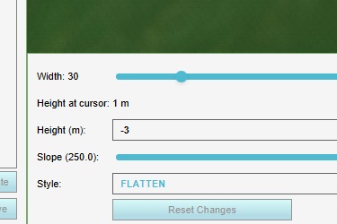
Configure the brush as follows (approximately): | |||
* Width: 30 (meter) | |||
* Height: -3 (meter) | |||
* Slope: 250 | |||
* Style: Flatten | |||
This will create a hole, with a radius of 30 meters, and a depth of 4 meters. (The project area's default height is 1 meter above datum, and the specified setting will place the bottom of the hole at 3 meters below {{datum}}, so the total depth will be 4 meters) | |||
[[File:Testbed_ElevationBrush1.jpg|350px|frame|center|Settings for the first manipulation of the terrain.]] | |||
In the [[3D Visualization]], click anywhere in the [[project area]], such that the entire hole is inside the project area. (If you are having trouble determining where the edge of your project area is, try placing a construction in the corner of the project first, as a navigational aid. Adding a construction will not affect the model we are setting up.) | |||
[[File:Testbed_ElevationBrush2.jpg|350px|frame|center|The first manipulation of the terrain.]] | |||
''Note that the hole created may appear to be filled with water. This is because the selection made is not permanent yet. As a result, the water visualization has not been updated yet, and may appear whenever a selection which lowers terrain is made.'' | |||
{{page_break}} | |||
If the created selection is as desired, please feel free to apply selection before you start drawing a new selection. Take into account that there is no undo option so the applied selection is permanent. Next, change the "height" setting of the brush to -6. | |||
[[File:Testbed_ElevationBrush3.jpg|350px|frame|center|Change the height setting.]] | |||
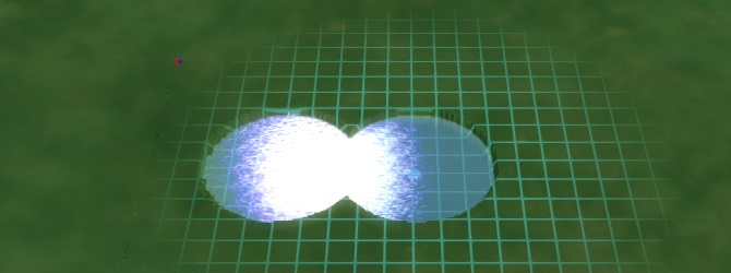
Now place another hole in the project area, such that the first hole and the second hole are connected. | |||
[[File:Testbed_ElevationBrush4.jpg|350px|frame|center|The two holes overlap.]] | |||
{{page_break}} | |||
Finally, click "Apply Changes" to complete the adjustment of the terrain height. | |||
[[File:Testbed_ElevationBrush5.jpg|350px|frame|center|The selection so far is a preview of the manipulation you wish to make. When you click "Apply", the changes are actually made.]] | |||
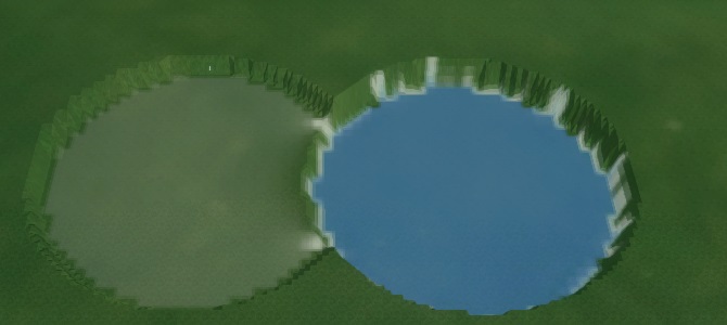
Now that the heightmap is changed, you will be able to properly see the created holes. | |||
[[File:Testbed_ElevationBrush6.jpg|350px|frame|center|When the actual change is applied, the water visualization is redetermined as well, showing the actual terrain height.]] | |||
Now we have a basic height difference. The reason for creating 2 pits instead of 1, is to make sure that water which is used in this test remains in this test, and does not flow of into other places. If water is allowed to flow away, then at least its not possible to account for all the water in the end result, and at worst the water may affect other tests. | |||
{{page_break}} | |||
Add an area to the project. Set the name of the area to "Inundation 1". | |||
[[File:AddArea.jpg|350px|frame|center|Add an area to the project.]] | |||
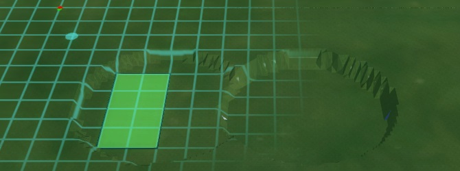
Draw the area in the project area. Specifically, make sure it sits inside the higher of the 2 hole, with no edges on the normal surface. | |||
[[File:Testbed_Area1.jpg|350px|frame|center|The location where the area is drawn will be filled with a column of water.]] | |||
{{page_break}} | |||
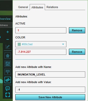
Add the attribute "INUNDATION_LEVEL" to the area, with a value of "-1". In the context of the flooding overlay, this means this area has a column of water up to the height of -1 meter relative to datum. The bottom of the hole being at -3 meters relative to datum, the column of water will be 2 meters high, but still 2 meters below the surface of the rest of the terrain. | |||
[[File:Testbed_Area2.jpg|350px|frame|center|The INUNDATION_LEVEL attribute will be interpreted by the flooding overlay as an initial deposit of water.]] | |||
Looking at the current result of the calculation of the flooding overlay, it's clear that the results are rather crude. Therefore the results on your screen can differ from the image you so in this tutorial. By changing the grid size the results will probably corresponde better accordingly to this image. | |||
[[File:Testbed_WaterResult1.jpg|350px|frame|center|The results do not yet display intuitively recognizable information.]] | |||
This is due to 2 default configurations for the flooding overlay, namely the grid cell size affecting how accurate the results are, and the result type which affects what the results are. | |||
{{page_break}} | |||
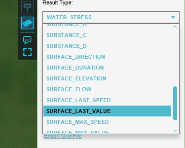
Currently, the result type is WATER_STRESS, which shows the highest amounts of water which existed in a cell at any point during the overlay's calculation. Set the result type to SURFACE_LAST_VALUE, which shows the exact amount of water present in any cell at any given point in the calculation. | |||
[[File:Testbed_ResultType.jpg|350px|frame|center|Change the result type to SURFACE_LAST_VALUE to get a more intuitive output.]] | |||
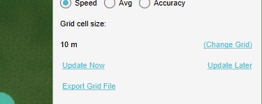
Next, select "Change Grid". | |||
[[File:Testbed_Grid1.jpg|350px|frame|center|The "Change Grid" option allows changing the accuracy of the calculation and its results.]] | |||
{{page_break}} | |||
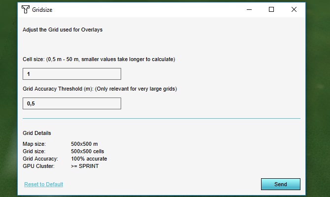
Change the grid cell size settings as follows: | |||
* Cell size: 1 meter | |||
* Grid accuracy threshold: 0.5 meter | |||
This will greatly increase the accuracy of the calculation. Due to the simplicity of the model, the calculation times will still be extremely low. | |||
[[File:Testbed_Grid2.jpg|350px|frame|center|Set the grid parameters to lower values to increase their accuracy.]] | |||
Click "Send". After the overlay has recalculated, you will see the end result of the flooding calculation has changed. | |||
[[File:Testbed_WaterResult2.jpg|350px|frame|center|The results are more accurate now]] | |||
{{page_break}} | |||
Use the timeframe controls in the overlay's legend to switch to the first timeframe. | |||
[[File:Testbed_LegendControls1.jpg|350px|frame|center|The timeframe controls of the overlay can be used to switch between various snapshots made during the calculation.]] | |||
What you'll notice specifically is that the calculation's results is composed of 10 timeframes. Each of the timeframes represents a snapshot of the process of water flowing into the deeper hole. However, the water flows so quickly that even at the first timeframe most water has already flowed into the lower hole. This means the timescale of the simulation should be tweaked as well. | |||
Select the overlay in the editor, and open the configuration wizard. | |||
[[File:Testbed_ConfigurationWizard1.jpg|350px|frame|center|The configuration wizard allows for easily configuring a number of parameters for the calculations.]] | |||
{{page_break}} | |||
Click "Next" to continue to the weather configuration step. In this step, set the following configuration: | |||
* Rain for 0 minutes | |||
* Total rainfall 0 mm | |||
* 0 days, 0 hours, 10 minutes dry after rain | |||
* Surface evaporation of 0 mm/day | |||
[[File:Testbed_ConfigurationWizard2.jpg|350px|frame|center|Rainfall, simulation time, and evaporation rate. Each of these properties have default values which can and should be tweaked to have better control over what happens during the calculation.]] | |||
Close the configuration wizard, and click "Update Now" to force the overlay to recalculate. | |||
Now using the timeframe controls, its possible to see how the water moves into the lower hole over time. | |||
[[File:Testbed_WaterResult2TimeframeControls.jpg|350px|frame|center|The final result of the calculation, but other timeframes show other moments during the calculation in which different amounts of water have had a chance to flow.]] | |||
This setup demonstrates basic water flow, namely that water will flow from a higher region to a lower region. It also shows that a small amount of water may be left behind, which can be explained either by friction, or by the flow of water also being dictated by the height of the water column. | |||
{{page_break}} | |||
===Culvert flow=== | |||
A slightly more complex setup is one where the 2 holes aren't directly connected to one another, but via a culvert set at a specific height. | |||
Note that we will not clear out the previous setup from the project. We will add this setup in parallel to the first one. | |||
Open the terrain elevation tool again. Configure the brush as follows: | |||
* Width: 30 (meter) | |||
* Height: -3 (meter) | |||
* Slope: 250 | |||
* Style: Flatten | |||
Next, pick a new location for another setup, without it overlapping with the first setup. Click in the 3D Visualization to create a new hole. Create another hole next to it, in such a way that there is still some room between them. Both holes should now be identical. | |||
[[File:Testbed_ElevationBrush7.jpg|350px|frame|center|The two created holes are separate from the first setup, and are separate from one another.]] | |||
Add another area to the project, and name it "Inundation 2". Draw it in so it completely covers one of the newly created holes. | |||
[[File:Testbed_Area3.jpg|350px|frame|center|The entire hole will be filled with water. Water will not be placed on the default land, as the height of the water will be set to be below the height of the terrain.]] | |||
{{page_break}} | |||
Add the attribute "INUNDATION_LEVEL" attribute to the area, and set the value to -1. | |||
[[File:Testbed_Area2.jpg|350px|frame|center|Set the INUNDATION_LEVEL attribute.]] | |||
Now when the overlay is recalculated, the results will show the hole is now filled with water, without having flowed into the other hole. | |||
[[File:Testbed_WaterResult3.jpg|350px|frame|center|One of the holes is filled with water.]] | |||
It is certain that the terrain elevation does not allow water to flow from one hole to another. This is good, because that means that when a culvert is added, it is the only way via which water can flow. The results will therefor be entirely dictated by the culvert's flow. | |||
{{page_break}} | |||
Add an underground construction to the project. | |||
[[File:AddUndergroundConstruction.jpg|350px|frame|center|Add an underground construction.]] | |||
Select the construction. Click on the "Change Function" button to open the function selection window. | |||
[[File:UndergroundConstructionChangeFunction.jpg|350px|frame|center|Click on "Change Function" to change the function of the construction.]] | |||
{{page_break}} | |||
Select the "Culvert" function, and then click "Apply". | |||
[[File:UndergroundConstructionChangeFunctionCulvert.jpg|650px|thumb|center|Find and select the "Culvert" function.]] | |||
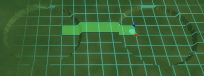
Draw the culvert into the project area, such that each end is inside one of the holes. | |||
[[File:Testbed_DrawConstruction2.jpg|350px|frame|center|Make sure each end is at least one full block inside the hole.]] | |||
{{page_break}} | |||
When the culvert is added to the project, and the overlay is recalculated, the effect of the presence of a culvert is already apparent, with water having flowed into the other hole. | |||
[[File:Testbed_WaterResult4.jpg|350px|frame|center|The second hole now also contains water.]] | |||
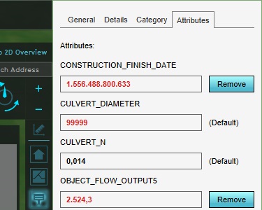
Since the only aspect of interest for this setup is the height at which the culvert exists, it's necessary to rule out the limiting effect culverts would have on throughput. Switch to the culvert's "Attributes" tab, and change the "CULVERT_DIAMETER" attribute to 99999. | |||
[[File:Testbed_ConstructionAttribute3.jpg|350px|frame|center|By increasing the diameter of the culvert, the effect of limited throughput through the culvert is disregarded.]] | |||
{{page_break}} | |||
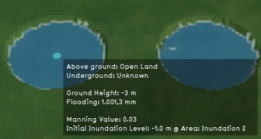
After the overlay recalculates, you can click in either hole and see the calculated water level. Both water columns should be around the same height, to within a few centimeters of margin. | |||
[[File:Testbed_WaterResult5.jpg|350px|frame|center|Clicking in either hole will show comparable values.]] | |||
Now, the height of the culvert can be configured. Add the attribute "CULVERT_THRESHOLD" attribute to the culvert, with the value "-1,5". | |||
[[File:Testbed_ConstructionAttribute4.jpg|350px|frame|center|The "CULVERT_THRESHOLD" attribute effectively sets the height at which the culvert resides.]] | |||
The result now is that water flows from one hole to another, via a culvert at a height of -1.5 meters relative to {{datum}}. The height of the water starts at -1 meters relative to {{datum}}. Water flows through the culvert, lowering the height of the water, until the water level passes the bottom of the culvert. From that point onward, water can no longer flow through the culvert, and thus the water level stops decreasing. | |||
[[File:Testbed_WaterResult6.jpg|350px|frame|center|All the water that sits below the culvert cannot flow through the culvert.]] | |||
Now using the timeframe controls, its possible to see how the water moves into the lower hole over time. Most notably, that the flow of water explicitly stops when the water level gets below the height of the culvert. | |||
{{page_break}} | |||
This setup demonstrates that water will flow from a location with a higher water level to a location with a lower water level, if there is a path the water can take. If a construction allows water to flow through and the water level is high enough to reach it, water can and will flow through. When that is no longer true, the flow of water stops. | |||
{{page_break}} | |||
===Simultaneous flow network=== | |||
Besides setups in which a single aspect is highlighted by itself, the knowledge of how one or more elements function can be brought together, to see if their combined behavior behaves as you may expect. The situation we are going to model will have a start basin which holds the initial store of water. Connected to it will be the main water basin which is slowly filled with water from the initial storage basin. Two outflow basins will be connected to the main water basin. The outflow basins will be connected via culverts at differing heights, so the setup demonstrates how the flow of water can be predicted based on the potential throughput of elements in other parts of the water system. | |||
Open the terrain elevation tool again. Configure the brush as follows: | |||
* Width: 30 (meter) | |||
* Height: -3 (meter) | |||
* Slope: 250 | |||
* Style: Flatten | |||
Next, pick a third location for another setup, without it overlapping with the previous setups. Click in the 3D Visualization to create a new hole. This will be the initial water store. | |||
[[File:Testbed_ElevationBrush8.jpg|350px|frame|center|Place the first hole for this setup, not too close to the existing setups because this setup will require a tiny bit more space.]] | |||
Change the "height" setting of the brush to -6, and place another hole next to the first hole, such that they are not directly connected. This will be the main water basin. | |||
[[File:Testbed_ElevationBrush9.jpg|350px|frame|center|Place the second hole near the first hole.]] | |||
{{page_break}} | |||
Change the "height" setting of the brush to -10, and place 2 more holes next to the second hole. These will be the outflow basins. | |||
[[File:Testbed_ElevationBrush10.jpg|350px|frame|center|Two additional holes.]] | |||
Finally, if you haven't done so yet, apply the selection so the holes are created. | |||
Add another area to the project, and name it "Inundation 3". Draw it in so it completely covers the first hole created; the initial water store. | |||
[[File:Testbed_Area4.jpg|350px|frame|center|Again draw in a new inundation area.]] | |||
Add the attribute "INUNDATION_LEVEL" attribute to the area, and set the value to 0. | |||
[[File:Testbed_Area5.jpg|350px|frame|center|This will fill the hole with a water column with a height of 3 meters.]] | |||
{{page_break}} | |||
Add a culvert to the project area, connecting the first 2 holes; the initial water basin and the main water basin. | |||
[[File:Testbed_DrawConstruction3.jpg|350px|frame|center|A culvert connecting the basins.]] | |||
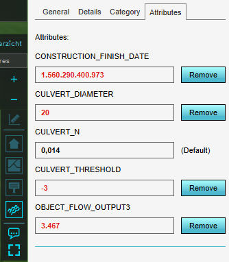
Set the following attributes for the culvert: | |||
* CULVERT_THRESHOLD: -3 | |||
* CULVERT_DIAMETER: 20 | |||
Leave the other attributes as they are. | |||
[[File:Culvert_specs.png|350px|frame|center|The attributes for the culvert.]] | |||
{{page_break}} | |||
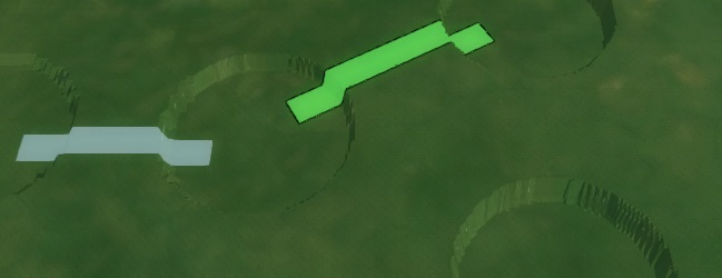
Add a culvert to the project area, connecting the second hole to one of the last 2 holes; a connection between the main water basin and an outflow basin. Give the culvert the following attributes: | |||
* CULVERT_THRESHOLD: -5 | |||
* CULVERT_DIAMETER: 1 | |||
Leave the other attributes as they are. | |||
[[File:Testbed_DrawConstruction4.jpg|350px|frame|center|The second culvert. If it's necessary to draw the culverts at an angle, you can use the "Line" draw mode.]] | |||
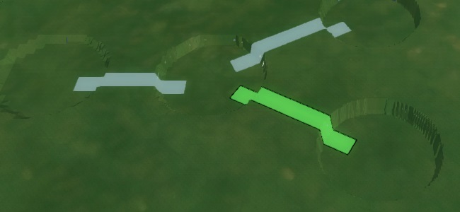
Add a culvert to the project area, connecting the second hole to the other of the last 2 holes; a connection between the main water basin and the remaining outflow basin. Give the culvert the following attributes: | |||
* CULVERT_THRESHOLD: -4 | |||
* CULVERT_DIAMETER: 6 | |||
Leave the other attributes as they are. | |||
[[File:Testbed_DrawConstruction5.jpg|350px|frame|center|The last culvert.]] | |||
{{page_break}} | |||
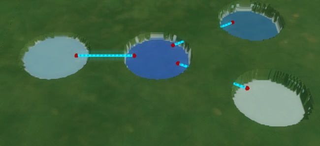
This setup will mean that water flows into the main water basin. Some water will flow into the first outflow basin, but its culvert does not have sufficient capacity to drain water from the main water basin as fast as it is being filled. At a certain point the water level in the main water basin is so high that water begins to flow into the second outflow basin. When the flow into the main water basin tapers off, flow into the second outflow basin should stop as well, leaving only the first outflow basin to be slowly filled with the remaining water. | |||
[[File:Testbed_WaterResult7.jpg|350px|frame|center|The final state of the water after the water calculation completes.]] | |||
{{page_break}} | |||
===Result analysis with the measuring tool=== | |||
The project now has a number of functionality demonstrations. Visually, it is easy to get an initial sense of what happens where. However, some subtle details in what happens during the simulation may not be immediately evident. To get a greater insight into how the water flow progresses, the measuring tool is especially useful. | |||
In the overlay menu, select the measuring tool icon. It is located directly above the overlay icons, and directly below the camera controls. | |||
[[File:Testbed_MeasurementTool.jpg|350px|frame|center|Click the measuring icon to open the measuring tool.]] | |||
The measuring tool now opens. This tool allows measurement points to be placed in the 3D Visualization. These measurement points give insight into the results of calculated overlays. | |||
[[File:Testbed_MeasurementTool2.jpg|350px|frame|center|The measuring tool.]] | |||
{{page_break}} | |||
With the measuring tool open, and with the flooding overlay active, click in any of the basins with water to place a measuring point. This will show a graph of how much water is calculated to be in that basin at any given point during the calculation. | |||
[[File:Testbed_MeasurementTool3.jpg|350px|frame|center|Results of a measuring point.]] | |||
The measuring tool works on any calculated overlay, so the magnitudes and units of the values displayed are dependent on the selected overlay. In the case of the flooding overlay used here, it displays the height of the water column in meters, relative to the surface of the terrain. | |||
{{page_break}} | |||
Using the tool, it's possible to inspect more closely what happens in the flow network. Place the measuring point in the main water basin of the flow network. | |||
[[File:Testbed_MeasurementTool4.jpg|350px|frame|center|Height of the water column in the flow network setup.]] | |||
This will show that over time, water will flow into the water basin. But the water levels off at a certain point, indicating that the inflow and outflow are in balance. This continues up to a certain point, where the water level begins to lower, meaning the inflow is decreasing, while outflow continues. | |||
{{page_break}} | |||
{{header|level=3|color=#c45911|Assignments}} | |||
These assignments reinforce the use of measurements and deduction to gain knowledge from a testbed. | |||
# Place measuring points in the outflow basins, and find the correlation between the graphs displayed in this way, and the graph of the main water basin. | |||
# Change the TIMEFRAMES attribute of the flooding overlay to 30, so more snapshots are made during the simulation. Place measuring points in the basins again and inspect the water flow in more detail. | |||
# Set up an additional demonstration of 2 water basins connected by a weir. Set the weir height (WEIR_HEIGHT) to the same value as the culvert in the comparable setup made during the tutorial. Compare the speed at which water flows in this setup with the culvert setup. | |||
{{Tutorial completed | |||
| learned=how to create testbeds, and use empty projects for experimentation | |||
}} | |||
Latest revision as of 14:14, 30 January 2023
Prerequisites
The following prerequisites should be met before starting this tutorial:
- This tutorial relies on base knowledge about the editor interface. If you have not yet followed the tutorials related to those subjects please do so first.
- This tutorial can be followed in an empty project area.
- Knowledge of the functioning of the water module is recommended, but not required.
Preparations
Take the following steps as preparation for following this tutorial:
- Create a new, empty project, sized to 500m by 500m. Ensure the unit system is set to "International". Also ensure it's an empty project area, not based on a real world location.
Introduction to testbeds
A testbed is a controlled setup, in which there are as few variables as possible which could influence a given situation.
In the Tygron Platform, whenever you create a project based on real-world data, the project is populated with a wide range of data. Virtually every project area contains numerous constructions, height differentials, and terrain types. If any calculation takes place, especially spatial calculations, all that data can serve as input. That makes it a lot more difficult to see exactly how a specific element factors into a specific result, or where the difference between an expected and actual result comes from.
Testbeds can serve the following purposes:
- Quick investigations into how a specific functionality works
- Demonstrations of multiple functionalities
- Forming a baseline for consistency testing
- Testing for (and demonstrations of) bugs or other issues
For this reason, what characterizes a testbed most is the absence of data. Anything that is not required for a specific case is left out, or at least left in a uniform, invariable state.
Starting point
For each testbed, the starting point is the empty project.
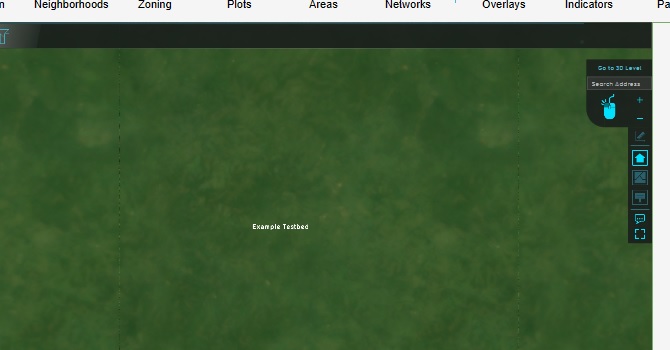
An empty project contains the following data:
- There is a uniform height map, with the height of the terrain set to 1m relative to datum.
- The surface of the terrain is the "Open Land" type. The underground terrain is the "Unknown" type.
- There is only a single municipal stakeholder, as a stakeholder to select for an editing user. The entirety of the project area is owned by that stakeholder.
- There are 4 neighborhoods (north-west, north-east, south-west, south-east), or if the project area is small, 1 single neighborhood.
- There is no zoning plan.
- There are no construction.
- The upper-left spatial coordinates of the project area are set to 0 degrees latitude and longitude.
Quick functionality testing
Testbeds can be used to test specific implementation questions. The question you're going to investigate is how the average overlay calculation functions in cases where the calculation takes place near the edge of the project area.
The average overlay functions, for any given grid cell, by looking at the surrounding grid cells, calculating the average value of the cells found. In most locations in a project area this calculation is very straightforward. However, if any of the cells looked at would fall outside the project area, any number of behaviors could be reasonable. For example: the cells outside the project area could be assumed to have a certain default value, or the cells could be disregarded for the calculations. You will configure the testbed to reveal how the average overlay deals with cells outside the project area.
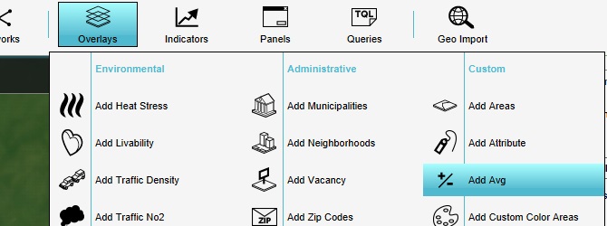
Start by adding the overlay we're going to test. Add an average overlay to the project.
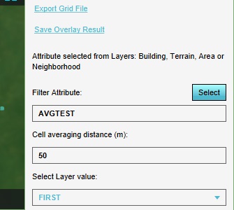
Prepare the overlay in such a way that it will calculate the spatial average of a user-defined attribute. As Filter Attribute, enter "AVGTEST" in the General tab in the right panel. Also set the Cell averaging distance to 50m. This will ensure that multiple entities can be drawn in the map and be spatially calculated, without necessarily affecting each other's outcomes.
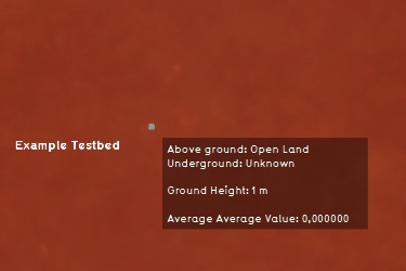
With this configuration, the calculation will result in a value of 0 in every location.
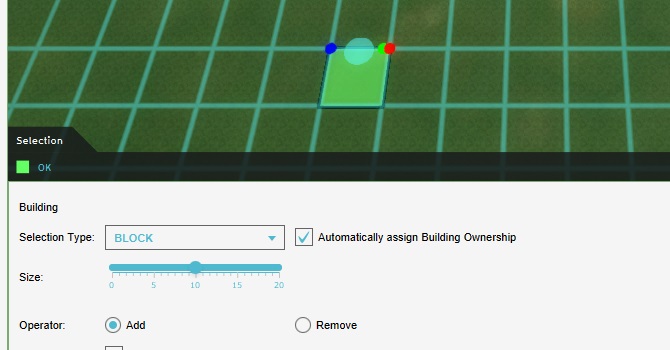
Now add a construction to the project, and place it more or less in the center of the project. Make sure you use the block-based brush, and draw in exactly 1 block (10m by 10m, for a total of 100m²).
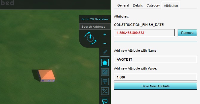
Add an AVGTEST attribute to the construction, with a value of 1000.
Switch back to the average overlay in the editor, and select "Update Now" to recalculate the content
Now, if you open the average overlay, you will see the construction is the center of a large area where the average value of AVGTEST is higher than in all other locations in the project area.
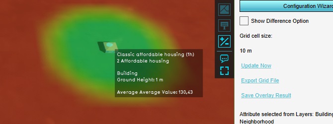
This setup creates a first look into how the average overlay functions. In the exact location of the construction, and its direct surroundings, the average value of AVGTEST is around 130. It tapers of at a distance of about 50 meters.
Note that you may see a value lower than 130, based on the exact location you have placed the construction. This is due to the construction's alignment on the calculation grid. This is expected, and does not affect the principles explained next. Take note of the value you see in your project, and continue.
We can now add another construction to the project, again with an AVGTEST attribute set to a value of 1000, and place that construction in the corner of the project area. Again, making sure that the construction is exactly 1 block of 10m by 10m, for a total of 100m².
Recalculating the overlay and looking at the average value at the location of the new construction gives an average value of 180.
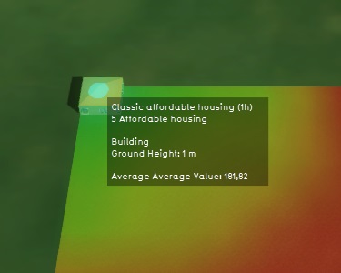
The fact that the calculated value in the corner is higher indicates that the cells outside the project area don't have an assumed value of 0 or lower.
Increase the AVGTEST attribute value of both constructions to 2000, and check again what average values are calculated in the locations of the constructions.
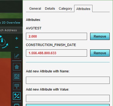
Now when you look at the calculated average value at the location of the construction, you will see that after doubling the attribute of the construction, the calculated value has doubled as well (give or take a rounding).
We can now put the following facts together:
- An average is a value calculated as follows: The sum of all values found in the calculation area, divided by the calculation area.
- The calculated average scales linearly with the value of the object we place. This means that the cells outside the project area do not have a positive or negative value. If they did, the impact of raising or lowering the attribute value would have been more or less impactful.
- An object at the edge of the project area has a greater impact on the calculated spatial average than a construction in the middle of the project area. This means that either the sum of all values increases as we get closer to the edge, or the surface area we divide by decreases.
We can determine that because the summed value does not change, the surface area used in the calculation must decrease in order to see the higher result. Thus our conclusion is that potential cells outside the project area are not used in the calculation of a spatial average.
Considerations
Note that based on the conclusion we have drawn, you may be tempted to expect the calculated values to match more neatly. Specifically, if the construction in the middle of the map has a full circle around it in which to perform its calculation, the construction in the edge of the map must have a quarter of the area of similar circle, thus the values should differ by a factor of 4. However, due to the layout of the constructions on the grid this is not the case.
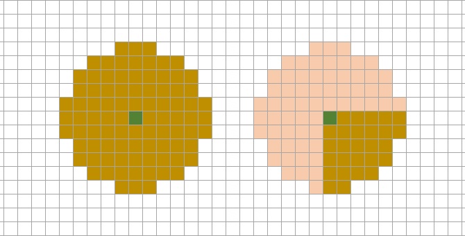
Also note that based on the exact size, placement, and rounding of values and polygons, it may be difficult to derive the outcomes seen from the base values without greater insight into the exact interpretations the Tygron Platform makes. This is to be expected, and the approach used here functions regardless of those exact calculations.
Assignments
These assignments are designed to demonstrate further means of experimentation.
- Knowing the radius of the spatial calculation is 50m, place a construction with the same attribute and value as close to the edge of the map as possible without the calculated average value differing from the construction in the middle of the project area.
- Change the average attribute of the constructions back to 1000, and instead expand both constructions with another block of 10m by 10m. Both constructions should be exactly twice as large as they were.
- Knowing the grid cell size is exactly 10m by 10m, find an explanation for the fact that both 'sides' of the construction in the middle of the map have the same calculated average, but the sides of the construction in the corner of the map do not.
Calculation insights
Testbeds, due to their inherent simplicity, can in some cases also be used to retrace exact calculations. The question you're going to investigate now is the size of the inactive border of the flooding overlay's calculation.
The calculation occurs in a grid, but the outer edge of grid cells is inactive. This means that there may be a discrepancy between input for the calculation and the results seen. If the exact number of cells can be determined, this discrepancy can be accounted for.
Either create a new empty project with the same specifications as in the prerequisites, or clean up the project configured during the last assignment by removing the added overlay and construction. Either way, make sure you start with an empty project area again.
Start by adding the overlay we are going to test. Add a flooding overlay to the project.
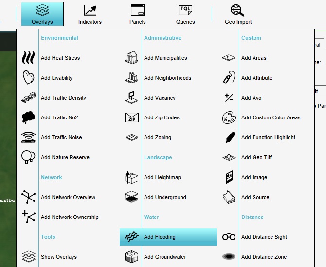
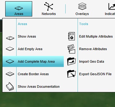
Add an area to the project, covering the complete project area.
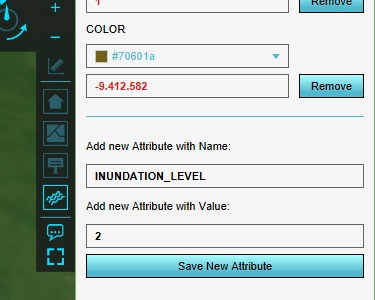
Add an INUNDATION_LEVEL attribute to the area, set to a value of 2.
This area will now cause the flooding overlay to initialize the calculation with a layer of 1 meter of water across the entire project area. (The project area's default height is 1 meter above datum, and the height of the water will be set to 2 meters above datum.)
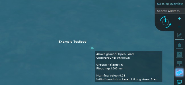
Activate the flooding overlay, and notice the entire project area is colored blue, indicating the presence of water. Click anywhere in the project area to see a "Flooding" height of 1 meter is calculated. If needed please make sure to calculate the area and overlay with the recalculate button in the upper left corner.
Select the flooding overlay in the editor, and select the "Show Water Balance" option.

The water balance opens. This window shows the amount of water in the project area, according to the flooding overlay's calculation.
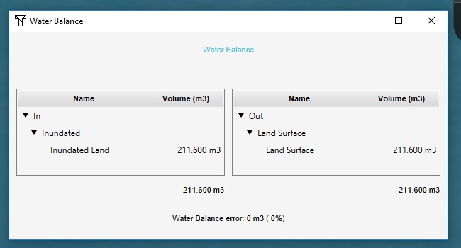
A project area of 500 meters by 500 meters has a total surface area of 250.000m². Given that the project area is covered uniformly by a layer of water of exactly 1 meter, this should result in 250.000m³ of water. However, the water balance indicates 211.600m³ of water in the project area. So there's 38.400m³ of water missing.
If you click at the edge of the project area, you will see that there is a zone where the amount of water is 0. This means that there are indeed cells where, despite covering the entire area uniformly with water, an edge of cells is excluded.
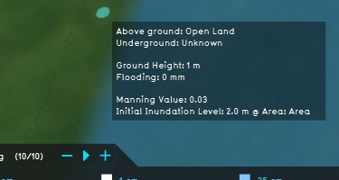
Knowing how large our project area is, and how much water is actually placed in the project area, we can calculate the amount of cells the project area is divided into, and the amount of cells which are actually used.
To calculate the amount of cells in the project area, we can take the size of the map (500 meters by 500 meters) and divide it by the grid cell size (which is 10 meters by 10 meters, by default). This tells us the project area is divided into 50 by 50 = 250 cells.
To calculate the amount of cells actually used in the project area, we work backward from the amount of water in the project. There is 211.600m³ of water, which means an area of 211.600m² is actually being calculated. Taking the square root of 211.600m², we get an active project area of 460 meters by 460 meters. This means 46 by 46 cells.
From this, we can conclude that the outer 2 cells are disregarded when performing the flooding overlay's calculations. (Along the horizontal axis, 2 cells on the west side and 2 cells on the east side are not used, and along the vertical axis 2 cells on the north side and 2 cells on the south side are not used.)
Model functionality demonstration
Testbeds can also be used to give an overview of multiple aspects of a model or functionality. These testbeds can take on the form of a single project with multiple isolated setups, or of one larger interconnected system. The question you're going to investigate now is how the water overlay deals with height differences.
"Height" is a broad concept, which means there is no singular detail to highlight. Instead, the proper approach is to see how height affects a basic setup, and then expand from that basic setup into slightly more complex configurations. The intent is to create an effective sense of how height is taken into account.
Either create a new empty project with the same specifications as in the prerequisites, or clean up the project configured during the last assignment by removing the added overlay and area. Either way, make sure you start with an empty project area again.
Next, again make sure we have a flooding overlay for our project.

Direct flow
The most basic setup to create is one where water directly flows from a higher location to a lower location.
Open the terrain's change elevation tool. You will use this to change the height of the terrain to create the necessary setup.
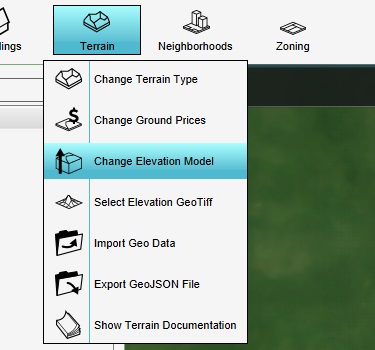
This will open the terrain elevation brush panel in the bottom of the editor. For simple setup, we will create 2 indentations in the terrain, directly attached to one another and one deeper than the other.
Configure the brush as follows (approximately):
- Width: 30 (meter)
- Height: -3 (meter)
- Slope: 250
- Style: Flatten
This will create a hole, with a radius of 30 meters, and a depth of 4 meters. (The project area's default height is 1 meter above datum, and the specified setting will place the bottom of the hole at 3 meters below datum, so the total depth will be 4 meters)
In the 3D Visualization, click anywhere in the project area, such that the entire hole is inside the project area. (If you are having trouble determining where the edge of your project area is, try placing a construction in the corner of the project first, as a navigational aid. Adding a construction will not affect the model we are setting up.)
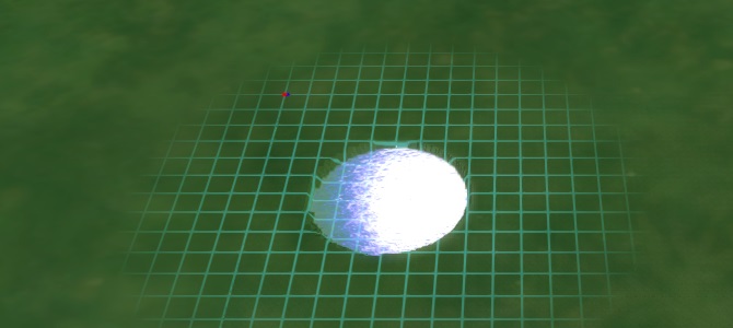
Note that the hole created may appear to be filled with water. This is because the selection made is not permanent yet. As a result, the water visualization has not been updated yet, and may appear whenever a selection which lowers terrain is made.
If the created selection is as desired, please feel free to apply selection before you start drawing a new selection. Take into account that there is no undo option so the applied selection is permanent. Next, change the "height" setting of the brush to -6.
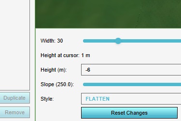
Now place another hole in the project area, such that the first hole and the second hole are connected.
Finally, click "Apply Changes" to complete the adjustment of the terrain height.
Now that the heightmap is changed, you will be able to properly see the created holes.
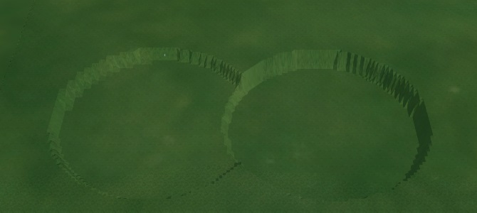
Now we have a basic height difference. The reason for creating 2 pits instead of 1, is to make sure that water which is used in this test remains in this test, and does not flow of into other places. If water is allowed to flow away, then at least its not possible to account for all the water in the end result, and at worst the water may affect other tests.
Add an area to the project. Set the name of the area to "Inundation 1".
Draw the area in the project area. Specifically, make sure it sits inside the higher of the 2 hole, with no edges on the normal surface.
Add the attribute "INUNDATION_LEVEL" to the area, with a value of "-1". In the context of the flooding overlay, this means this area has a column of water up to the height of -1 meter relative to datum. The bottom of the hole being at -3 meters relative to datum, the column of water will be 2 meters high, but still 2 meters below the surface of the rest of the terrain.
Looking at the current result of the calculation of the flooding overlay, it's clear that the results are rather crude. Therefore the results on your screen can differ from the image you so in this tutorial. By changing the grid size the results will probably corresponde better accordingly to this image.
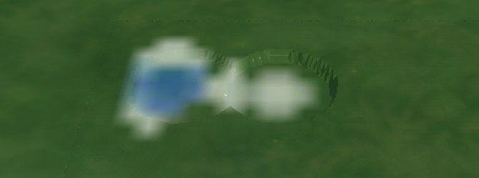
This is due to 2 default configurations for the flooding overlay, namely the grid cell size affecting how accurate the results are, and the result type which affects what the results are.
Currently, the result type is WATER_STRESS, which shows the highest amounts of water which existed in a cell at any point during the overlay's calculation. Set the result type to SURFACE_LAST_VALUE, which shows the exact amount of water present in any cell at any given point in the calculation.
Next, select "Change Grid".
Change the grid cell size settings as follows:
- Cell size: 1 meter
- Grid accuracy threshold: 0.5 meter
This will greatly increase the accuracy of the calculation. Due to the simplicity of the model, the calculation times will still be extremely low.
Click "Send". After the overlay has recalculated, you will see the end result of the flooding calculation has changed.
Use the timeframe controls in the overlay's legend to switch to the first timeframe.
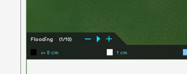
What you'll notice specifically is that the calculation's results is composed of 10 timeframes. Each of the timeframes represents a snapshot of the process of water flowing into the deeper hole. However, the water flows so quickly that even at the first timeframe most water has already flowed into the lower hole. This means the timescale of the simulation should be tweaked as well.
Select the overlay in the editor, and open the configuration wizard.
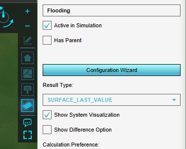
Click "Next" to continue to the weather configuration step. In this step, set the following configuration:
- Rain for 0 minutes
- Total rainfall 0 mm
- 0 days, 0 hours, 10 minutes dry after rain
- Surface evaporation of 0 mm/day
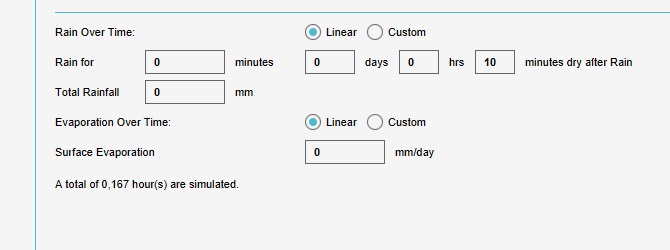
Close the configuration wizard, and click "Update Now" to force the overlay to recalculate.
Now using the timeframe controls, its possible to see how the water moves into the lower hole over time.
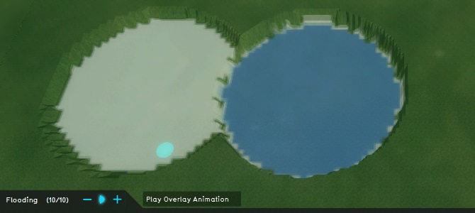
This setup demonstrates basic water flow, namely that water will flow from a higher region to a lower region. It also shows that a small amount of water may be left behind, which can be explained either by friction, or by the flow of water also being dictated by the height of the water column.
Culvert flow
A slightly more complex setup is one where the 2 holes aren't directly connected to one another, but via a culvert set at a specific height.
Note that we will not clear out the previous setup from the project. We will add this setup in parallel to the first one.
Open the terrain elevation tool again. Configure the brush as follows:
- Width: 30 (meter)
- Height: -3 (meter)
- Slope: 250
- Style: Flatten
Next, pick a new location for another setup, without it overlapping with the first setup. Click in the 3D Visualization to create a new hole. Create another hole next to it, in such a way that there is still some room between them. Both holes should now be identical.
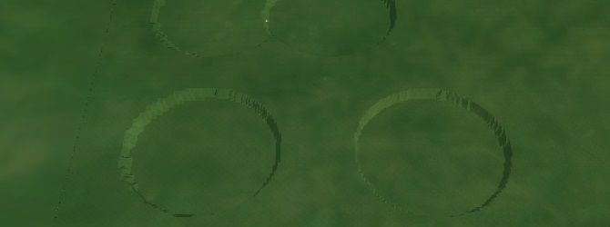
Add another area to the project, and name it "Inundation 2". Draw it in so it completely covers one of the newly created holes.
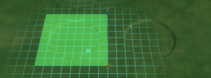
Add the attribute "INUNDATION_LEVEL" attribute to the area, and set the value to -1.

Now when the overlay is recalculated, the results will show the hole is now filled with water, without having flowed into the other hole.

It is certain that the terrain elevation does not allow water to flow from one hole to another. This is good, because that means that when a culvert is added, it is the only way via which water can flow. The results will therefor be entirely dictated by the culvert's flow.
Add an underground construction to the project.
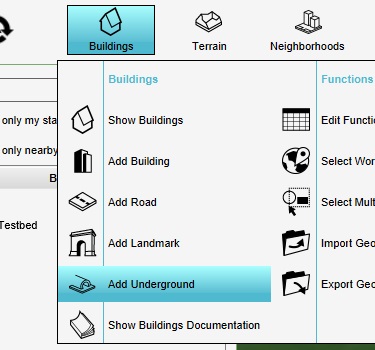
Select the construction. Click on the "Change Function" button to open the function selection window.
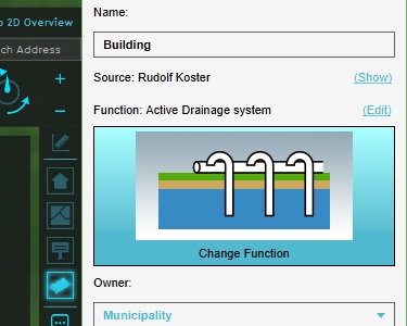
Select the "Culvert" function, and then click "Apply".
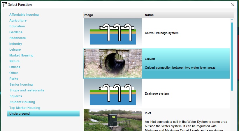
Draw the culvert into the project area, such that each end is inside one of the holes.
When the culvert is added to the project, and the overlay is recalculated, the effect of the presence of a culvert is already apparent, with water having flowed into the other hole.

Since the only aspect of interest for this setup is the height at which the culvert exists, it's necessary to rule out the limiting effect culverts would have on throughput. Switch to the culvert's "Attributes" tab, and change the "CULVERT_DIAMETER" attribute to 99999.
After the overlay recalculates, you can click in either hole and see the calculated water level. Both water columns should be around the same height, to within a few centimeters of margin.
Now, the height of the culvert can be configured. Add the attribute "CULVERT_THRESHOLD" attribute to the culvert, with the value "-1,5".
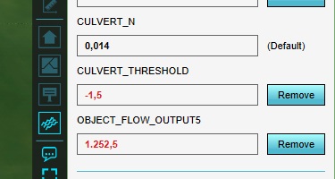
The result now is that water flows from one hole to another, via a culvert at a height of -1.5 meters relative to datum. The height of the water starts at -1 meters relative to datum. Water flows through the culvert, lowering the height of the water, until the water level passes the bottom of the culvert. From that point onward, water can no longer flow through the culvert, and thus the water level stops decreasing.

Now using the timeframe controls, its possible to see how the water moves into the lower hole over time. Most notably, that the flow of water explicitly stops when the water level gets below the height of the culvert.
This setup demonstrates that water will flow from a location with a higher water level to a location with a lower water level, if there is a path the water can take. If a construction allows water to flow through and the water level is high enough to reach it, water can and will flow through. When that is no longer true, the flow of water stops.
Simultaneous flow network
Besides setups in which a single aspect is highlighted by itself, the knowledge of how one or more elements function can be brought together, to see if their combined behavior behaves as you may expect. The situation we are going to model will have a start basin which holds the initial store of water. Connected to it will be the main water basin which is slowly filled with water from the initial storage basin. Two outflow basins will be connected to the main water basin. The outflow basins will be connected via culverts at differing heights, so the setup demonstrates how the flow of water can be predicted based on the potential throughput of elements in other parts of the water system.
Open the terrain elevation tool again. Configure the brush as follows:
- Width: 30 (meter)
- Height: -3 (meter)
- Slope: 250
- Style: Flatten
Next, pick a third location for another setup, without it overlapping with the previous setups. Click in the 3D Visualization to create a new hole. This will be the initial water store.
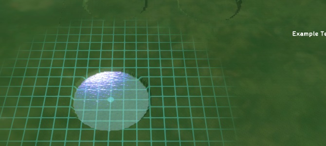
Change the "height" setting of the brush to -6, and place another hole next to the first hole, such that they are not directly connected. This will be the main water basin.

Change the "height" setting of the brush to -10, and place 2 more holes next to the second hole. These will be the outflow basins.
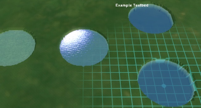
Finally, if you haven't done so yet, apply the selection so the holes are created.
Add another area to the project, and name it "Inundation 3". Draw it in so it completely covers the first hole created; the initial water store.

Add the attribute "INUNDATION_LEVEL" attribute to the area, and set the value to 0.
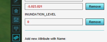
Add a culvert to the project area, connecting the first 2 holes; the initial water basin and the main water basin.

Set the following attributes for the culvert:
- CULVERT_THRESHOLD: -3
- CULVERT_DIAMETER: 20
Leave the other attributes as they are.
Add a culvert to the project area, connecting the second hole to one of the last 2 holes; a connection between the main water basin and an outflow basin. Give the culvert the following attributes:
- CULVERT_THRESHOLD: -5
- CULVERT_DIAMETER: 1
Leave the other attributes as they are.
Add a culvert to the project area, connecting the second hole to the other of the last 2 holes; a connection between the main water basin and the remaining outflow basin. Give the culvert the following attributes:
- CULVERT_THRESHOLD: -4
- CULVERT_DIAMETER: 6
Leave the other attributes as they are.
This setup will mean that water flows into the main water basin. Some water will flow into the first outflow basin, but its culvert does not have sufficient capacity to drain water from the main water basin as fast as it is being filled. At a certain point the water level in the main water basin is so high that water begins to flow into the second outflow basin. When the flow into the main water basin tapers off, flow into the second outflow basin should stop as well, leaving only the first outflow basin to be slowly filled with the remaining water.
Result analysis with the measuring tool
The project now has a number of functionality demonstrations. Visually, it is easy to get an initial sense of what happens where. However, some subtle details in what happens during the simulation may not be immediately evident. To get a greater insight into how the water flow progresses, the measuring tool is especially useful.
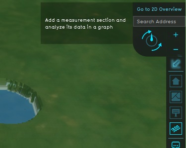
In the overlay menu, select the measuring tool icon. It is located directly above the overlay icons, and directly below the camera controls.
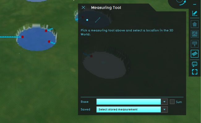
The measuring tool now opens. This tool allows measurement points to be placed in the 3D Visualization. These measurement points give insight into the results of calculated overlays.
With the measuring tool open, and with the flooding overlay active, click in any of the basins with water to place a measuring point. This will show a graph of how much water is calculated to be in that basin at any given point during the calculation.
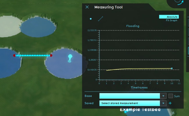
The measuring tool works on any calculated overlay, so the magnitudes and units of the values displayed are dependent on the selected overlay. In the case of the flooding overlay used here, it displays the height of the water column in meters, relative to the surface of the terrain.
Using the tool, it's possible to inspect more closely what happens in the flow network. Place the measuring point in the main water basin of the flow network.
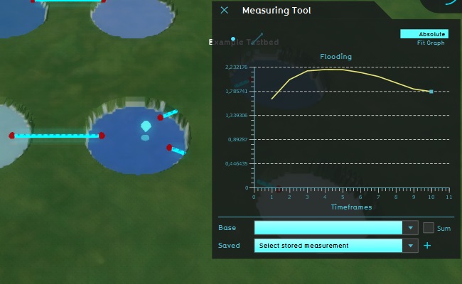
This will show that over time, water will flow into the water basin. But the water levels off at a certain point, indicating that the inflow and outflow are in balance. This continues up to a certain point, where the water level begins to lower, meaning the inflow is decreasing, while outflow continues.
Assignments
These assignments reinforce the use of measurements and deduction to gain knowledge from a testbed.
- Place measuring points in the outflow basins, and find the correlation between the graphs displayed in this way, and the graph of the main water basin.
- Change the TIMEFRAMES attribute of the flooding overlay to 30, so more snapshots are made during the simulation. Place measuring points in the basins again and inspect the water flow in more detail.
- Set up an additional demonstration of 2 water basins connected by a weir. Set the weir height (WEIR_HEIGHT) to the same value as the culvert in the comparable setup made during the tutorial. Compare the speed at which water flows in this setup with the culvert setup.
Tutorial completed
Congratulations. You have now completed this tutorial. In it, you have learned how to create testbeds, and use empty projects for experimentation.