Surface model (Water Overlay): Difference between revisions
No edit summary |
No edit summary |
||
| (31 intermediate revisions by 4 users not shown) | |||
| Line 1: | Line 1: | ||
__NOTOC__ | __NOTOC__ | ||
[[File:Waterlevel_schematic.png|300px|thumb|right|Fig. 1. For each grid cell:<br>''B'' = bottom elevation<br>''h'' = water depth<br>''w'' = water surface elevation]] | [[File:Waterlevel_schematic.png|300px|thumb|right|Fig. 1. For each grid cell:<br>''B'' = bottom elevation<br>''h'' = water depth<br>''w'' = water surface elevation]] | ||
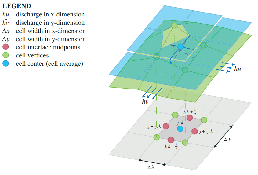
[[File:Inundation overlay 04 HWP(1).PNG|thumb|250px|Fig. 2. A 2-D grid-based representation of average water depths, discharges and bathymetry in a case where the middle cell is fully flooded in the y-dimension, but only partially flooded in the x-dimension. Blue solid and red dashed lines denote the waterlines and bathymetry slopes in both dimensions, respectively. For a bilinear reconstruction, the cell averages coincide with the values at the cell centers, while bathymetry is approximated by its values at the cell vertices. | [[File:Inundation overlay 04 HWP(1).PNG|thumb|250px|Fig. 2. A 2-D grid-based representation of average water depths, discharges and bathymetry in a case where the middle cell is fully flooded in the y-dimension, but only partially flooded in the x-dimension. Blue solid and red dashed lines denote the waterlines and bathymetry slopes in both dimensions, respectively. For a bilinear reconstruction, the cell averages coincide with the values at the cell centers, while bathymetry is approximated by its values at the cell vertices.{{ref|Horvath}}]] | ||
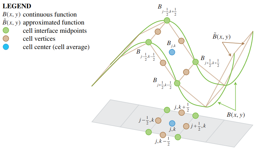
[[File:Inundation overlay 04 HWP(2).PNG|thumb|250px|Fig. 3. Continuous bathymetry function (green line) and its piecewise linear approximation (brown dots). The approximated function values equal to the continuous ones at the cell vertices (green dots). The cell average value (blue dot) equals both the average value of the vertex values (green dots) and the average value of the values at the cell interface midpoints (brown dots). | [[File:Inundation overlay 04 HWP(2).PNG|thumb|250px|Fig. 3. Continuous bathymetry function (green line) and its piecewise linear approximation (brown dots). The approximated function values equal to the continuous ones at the cell vertices (green dots). The cell average value (blue dot) equals both the average value of the vertex values (green dots) and the average value of the values at the cell interface midpoints (brown dots).{{ref|Horvath}}]] | ||
The [[Water Module]]'s primary function is simulating two-dimensional flow of water across the surface. In order to do this, the project area is first discretized into ''x'' by ''y'' cells depending on the configured [[grid cell size]]. Secondly, water is initialized in the model. Finally, a set of rules is required that describes the behavior of the flow. | The [[Water Module]]'s primary function is simulating two-dimensional flow of water across the surface. In order to do this, the project area is first discretized into ''x'' by ''y'' cells depending on the configured [[grid cell size]]. Secondly, water is initialized in the model. Finally, a set of rules is required that describes the behavior of the flow. | ||
===Surface flow scheme=== | ===Surface flow scheme=== | ||
In the model, imbalances in the water surface elevation across the grid drive the flow of water until a state of equilibrium is reached in terms of '' | In the model, imbalances in the water surface elevation across the grid drive the flow of water until a state of equilibrium is reached in terms of ''h'' and flux. Behavior of the flow is described by a second-order semi-discrete central-upwind scheme produced by Kurganov and Petrova (2007){{ref|Kurganov2}}, which is based on the 2-D Saint-Venant equations (a.k.a. shallow water equations): | ||
:<math> | :<math> | ||
| Line 30: | Line 12: | ||
\frac{\partial h}{\partial t} &+ \frac{\partial (hu)}{\partial x} + \frac{\partial (hv)}{\partial y} = 0,\\[3pt] | \frac{\partial h}{\partial t} &+ \frac{\partial (hu)}{\partial x} + \frac{\partial (hv)}{\partial y} = 0,\\[3pt] | ||
\frac{\partial (hu)}{\partial t} &+ \frac{\partial}{\partial x} \left( hu^2 + \frac{1}{2} gh^2 \right) + \frac{\partial (huv)}{\partial y} = -gh \frac{\partial B}{\partial x} - ghn^2u \sqrt{u^2 + v^2} h^{-\frac{4}{3}},\\[3pt] | \frac{\partial (hu)}{\partial t} &+ \frac{\partial}{\partial x} \left( hu^2 + \frac{1}{2} gh^2 \right) + \frac{\partial (huv)}{\partial y} = -gh \frac{\partial B}{\partial x} - ghn^2u \sqrt{u^2 + v^2} h^{-\frac{4}{3}},\\[3pt] | ||
\frac{\partial (hv)}{\partial t} &+ \frac{\partial (huv)}{\partial x} + \frac{\partial}{\partial y} \left( hv^2 + \frac{1}{2} gh^2 \right) = -gh \frac{\partial B}{\partial y} - ghn^ | \frac{\partial (hv)}{\partial t} &+ \frac{\partial (huv)}{\partial x} + \frac{\partial}{\partial y} \left( hv^2 + \frac{1}{2} gh^2 \right) = -gh \frac{\partial B}{\partial y} - ghn^2v \sqrt{u^2 + v^2} h^{-\frac{4}{3}}, | ||
\end{align} | \end{align} | ||
</math> | </math> | ||
| Line 45: | Line 27: | ||
| ''B'' || is the bottom elevation | | ''B'' || is the bottom elevation | ||
|- valign="top" | |- valign="top" | ||
| ''g'' || is | | ''g'' || is {{gravity}} | ||
|- valign="top" | |- valign="top" | ||
| ''n'' || is the Gauckler–Manning coefficient | | ''n'' || is the Gauckler–Manning coefficient | ||
|} | |} | ||
This scheme deviates from the original Saint-Venant equations in that it approaches the system in terms of water surface elevation (''w = h + B'') and flux (''hu'' and ''hv''), instead of just the water depth (''h''). The conceptual image in Fig. 1 aims to clarify on the various terms in the model equations. This method relies on a continuous piecewise linear approximation of the surface, which is further explained on [[Elevation model (Water Overlay)|this]] page. | This scheme deviates from the original Saint-Venant equations in that it approaches the system in terms of water surface elevation (''w = h + B'') and flux (''hu'' and ''hv''), instead of just the water depth (''h''). The conceptual image in Fig. 1 aims to clarify on the various terms in the model equations. This method relies on a continuous piecewise linear approximation of the surface, which is further explained on [[Elevation model (Water Overlay)|this]] page. | ||
This scheme is further extended with the shoreline reconstruction method by Bollerman et al (2014), which ensures better numerical stability at the wetting and drying fronts of a flood wave | ====Shoreline reconstruction==== | ||
This scheme is further extended with the shoreline reconstruction method by Bollerman et al (2014), which ensures better numerical stability at the wetting and drying fronts of a flood wave{{ref|Bollerman}}. An elaborate explanation is provided by Horváth et al. (2014){{ref|Horvath}}. | |||
General sequence of computational steps: | General sequence of computational steps: | ||
| Line 63: | Line 46: | ||
# Time is incremented with the calculated time step and changes in water level and fluxes are subsequently applied. | # Time is incremented with the calculated time step and changes in water level and fluxes are subsequently applied. | ||
== | ===Water level initialization=== | ||
In theory, each grid cell can have a unique bottom elevation and accompanying water depth, yielding a certain water surface elevation (or water level). However, in practice, water levels are often initialized for large groups of cells rather than individual cells, assuming that each (water level) area in a project has been assigned a [[water level (Water Overlay)|water level]]. During the initialization phase a distinction is made between two types: | |||
* [[water level (Water Overlay)|Water level]]s of [[Water area (Water Overlay)|water areas]]; | |||
* [[inundation level (Water Overlay)|Inundation level]]s of [[Inundation area (Water Overlay)|inundation areas]]. | |||
For all [[Terrain water (Water Overlay)|water terrain]]s in a water area, the volume of water per grid cell is such that the resulting water level at those locations conforms the value of the [[Water level (Water Overlay)|WATER_LEVEL]] attribute as provided by the corresponding [[Water area (Water Overlay)|water area]]. | |||
In contrast to water areas, which generate water on water terrains, inundation areas generate water over all grid cells, regardless of its terrain type. Similarly, the volume of water per grid cell is determined by the [[Inundation level (Water Overlay)|INUNDATION_LEVEL]] attribute as provided by the corresponding inundation area. | |||
If a grid cell is neither part of any water area nor inundation area, or the assigned water level is lower than its [[terrain height (Water Overlay)|bottom elevation]], the water depth is assumed to be zero and the water level becomes equal to the bottom elevation. In turn, this bottom (or surface) elevation is equal to the [[elevation model]], though it may be altered by the presence of a building or the [[Breach height (Water Overlay)|BREACH_HEIGHT]] attribute of a [[Breach (Water Overlay)|breach]]. | |||
===Water velocity initialization=== | |||
It is now also possible to initialize the [[Surface u prequel (Water Overlay)|velocity u]] and [[Surface v prequel (Water Overlay)|velocity v]] of surface water using [[Prequels (Water Overlay)|prequels]]. The [[Surface last u result type (Water Overlay)|surface u]] and [[Surface last v result type (Water Overlay)|surface v]] are also result overlays that can be inspected and used by subsequent simulations when stored and configured as prequels for other [[Water Overlay]]s. | |||
===Microrelief and minimum flow threshold=== | |||
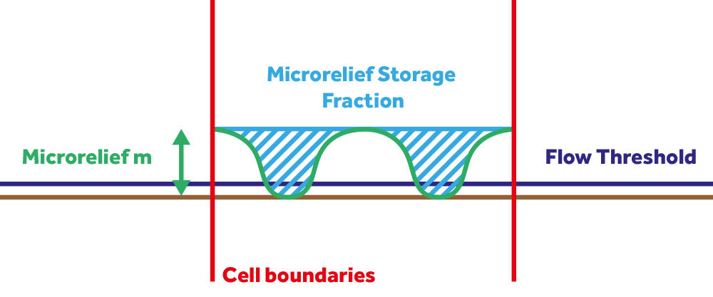
[[File:water_overlay_surface_model_microrelief_flow_threshold.png|thumb|right|[[Water microrelief m (Water Overlay)|Microrelief]], optional [[Microrelief storage fraction (Water Overlay)| microrelief storage fraction]] and the minimum flow threshold.]] | |||
For water to flow from a cell to its neighbors, the height of a water column needs to be at least 0.5mm. We call this the ''minimum flow threshold''. However, if microrelief is defined, this minimum flow threshold of a cell is potentially raised to the amount specified for microrelief. Microrelief can be specified by a function's [[Water microrelief m (Water Overlay)|microrelief]] or terrain's [[Terrain water microrelief m (Water Overlay)|microrelief]], or using a grid overlay for the [[Microrelief prequel (Water Overlay)|Microrelief prequel]]. Furthermore an optional [[Microrelief storage fraction (Water Overlay)|Microrelief storage fraction]] can be set, which will be applied to the microrelief threshold. | |||
{{article end | |||
|notes= | |||
* Water can be added to and removed from the described surface system by the [[Rain model (Water Overlay)|rain]], [[Evapotranspiration model (Water Overlay)|evapotranspiration]] and [[Infiltration model (Water Overlay)|infiltration model]], as well as certain [[Hydraulic structures (Water Overlay)|hydraulic structures]] and [[Breach (Water Overlay)|breach]]es. | |||
* In the case of [[Ground model (Water Overlay)|subsurface flow]] a different flow system with different equations are used. | |||
* In addition to water flowing in between grid cells, water can also flow ''through'' [[Hydraulic structures (Water Overlay)|hydraulic buildings]]. | |||
* The [[Design flood elevation m model attribute (Water Overlay)|DESIGN_FLOOD_ELEVATION_M]] attribute confines the maximum surface elevation induced by buildings. | |||
|references= | |||
<references> | <references> | ||
{{ref|Bollerman | |||
|name=A Well-balanced Reconstruction for Wetting, Drying Fronts. IGPM Report | |||
|author=Bollermann, Andreas & Chen, Guoxian & Kurganov, Alexander & Noelle, Sebastian. (2014) | |||
|page=313 | |||
|source= | |||
|link=https://www.researchgate.net/publication/269417532_A_Well-balanced_Reconstruction_for_Wetting_Drying_Fronts | |||
|lastvisit=2019-07-24 | |||
}} | |||
{{ref|Horvath | |||
|name=A two-dimensional numerical scheme of dry/wet fronts for the Saint-Venant system of shallow water equations | |||
|author=Zsolt Horváth, Jürgen Waser, Rui A. P. Perdigão, Artem Konev and Günter Blöschl (2014) | |||
|page= | |||
|source= | |||
|link=http://citeseerx.ist.psu.edu/viewdoc/download?doi=10.1.1.700.7977&rep=rep1&type=pdf, http://visdom.at/media/pdf/publications/Poster.pdf | |||
|lastvisit=2018-06-29 | |||
}} | |||
{{ref|Kurganov2 | |||
|name=A Second-Order Well-Balanced Positivity Preserving Central-Upwind Scheme for the Saint-Venant System | |||
|author=Kurganov A, Petrova G (2007) | |||
|page= | |||
|source= | |||
|link=http://www.math.tamu.edu/~gpetrova/KPSV.pdf | |||
|lastvisit=2019-04-11 | |||
}} | |||
</references> | </references> | ||
}} | |||
{{ | {{WaterOverlay formula nav}} | ||
Latest revision as of 14:39, 17 October 2025

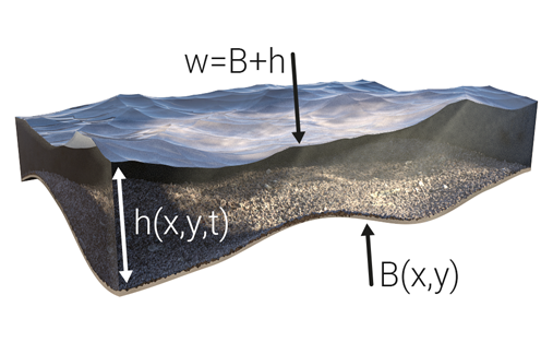
B = bottom elevation
h = water depth
w = water surface elevation


The Water Module's primary function is simulating two-dimensional flow of water across the surface. In order to do this, the project area is first discretized into x by y cells depending on the configured grid cell size. Secondly, water is initialized in the model. Finally, a set of rules is required that describes the behavior of the flow.
Surface flow scheme
In the model, imbalances in the water surface elevation across the grid drive the flow of water until a state of equilibrium is reached in terms of h and flux. Behavior of the flow is described by a second-order semi-discrete central-upwind scheme produced by Kurganov and Petrova (2007)[2], which is based on the 2-D Saint-Venant equations (a.k.a. shallow water equations):
where
u is the velocity in the x-direction v is the velocity in the y-direction h is the water depth B is the bottom elevation g is the acceleration due to gravity, set to 9.80665 n is the Gauckler–Manning coefficient
This scheme deviates from the original Saint-Venant equations in that it approaches the system in terms of water surface elevation (w = h + B) and flux (hu and hv), instead of just the water depth (h). The conceptual image in Fig. 1 aims to clarify on the various terms in the model equations. This method relies on a continuous piecewise linear approximation of the surface, which is further explained on this page.
Shoreline reconstruction
This scheme is further extended with the shoreline reconstruction method by Bollerman et al (2014), which ensures better numerical stability at the wetting and drying fronts of a flood wave[3]. An elaborate explanation is provided by Horváth et al. (2014)[1].
General sequence of computational steps:
- Each cell's elevation value (B in Fig. 3) is set equal to the value at its center and the interface midpoints.
- Slopes of conserved variables are reconstructed (continuity and momentum in x- and y-direction).
- Values of conserved variables at the cell interface midpoints are compared with the left-sided and right-sided values with respect to the cell's center.
- Slopes of partially dry cells are modified to prevent negative depth values and numerical instability.
- Fluxes are computed at each cell interface to determine the values of the conserved variable at the cell centers for the next time step.
- The largest allowed time step is calculated.
- Time is incremented with the calculated time step and changes in water level and fluxes are subsequently applied.
Water level initialization
In theory, each grid cell can have a unique bottom elevation and accompanying water depth, yielding a certain water surface elevation (or water level). However, in practice, water levels are often initialized for large groups of cells rather than individual cells, assuming that each (water level) area in a project has been assigned a water level. During the initialization phase a distinction is made between two types:
For all water terrains in a water area, the volume of water per grid cell is such that the resulting water level at those locations conforms the value of the WATER_LEVEL attribute as provided by the corresponding water area.
In contrast to water areas, which generate water on water terrains, inundation areas generate water over all grid cells, regardless of its terrain type. Similarly, the volume of water per grid cell is determined by the INUNDATION_LEVEL attribute as provided by the corresponding inundation area.
If a grid cell is neither part of any water area nor inundation area, or the assigned water level is lower than its bottom elevation, the water depth is assumed to be zero and the water level becomes equal to the bottom elevation. In turn, this bottom (or surface) elevation is equal to the elevation model, though it may be altered by the presence of a building or the BREACH_HEIGHT attribute of a breach.
Water velocity initialization
It is now also possible to initialize the velocity u and velocity v of surface water using prequels. The surface u and surface v are also result overlays that can be inspected and used by subsequent simulations when stored and configured as prequels for other Water Overlays.
Microrelief and minimum flow threshold

For water to flow from a cell to its neighbors, the height of a water column needs to be at least 0.5mm. We call this the minimum flow threshold. However, if microrelief is defined, this minimum flow threshold of a cell is potentially raised to the amount specified for microrelief. Microrelief can be specified by a function's microrelief or terrain's microrelief, or using a grid overlay for the Microrelief prequel. Furthermore an optional Microrelief storage fraction can be set, which will be applied to the microrelief threshold.
Notes
- Water can be added to and removed from the described surface system by the rain, evapotranspiration and infiltration model, as well as certain hydraulic structures and breaches.
- In the case of subsurface flow a different flow system with different equations are used.
- In addition to water flowing in between grid cells, water can also flow through hydraulic buildings.
- The DESIGN_FLOOD_ELEVATION_M attribute confines the maximum surface elevation induced by buildings.
References
- ↑ 1.0 1.1 1.2 A two-dimensional numerical scheme of dry/wet fronts for the Saint-Venant system of shallow water equations ∙ Zsolt Horváth, Jürgen Waser, Rui A. P. Perdigão, Artem Konev and Günter Blöschl (2014) ∙ Found at: http://citeseerx.ist.psu.edu/viewdoc/download?doi=10.1.1.700.7977&rep=rep1&type=pdf, http://visdom.at/media/pdf/publications/Poster.pdf ∙ (last visited: 2018-06-29)
- ↑ A Second-Order Well-Balanced Positivity Preserving Central-Upwind Scheme for the Saint-Venant System ∙ Kurganov A, Petrova G (2007) ∙ Found at: http://www.math.tamu.edu/~gpetrova/KPSV.pdf ∙ (last visited: 2019-04-11)
- ↑ A Well-balanced Reconstruction for Wetting, Drying Fronts. IGPM Report ∙ Bollermann, Andreas & Chen, Guoxian & Kurganov, Alexander & Noelle, Sebastian. (2014) ∙ Page(s): 313 ∙ Found at: https://www.researchgate.net/publication/269417532_A_Well-balanced_Reconstruction_for_Wetting_Drying_Fronts ∙ (last visited: 2019-07-24)


