Elevation model (Water Overlay): Difference between revisions
No edit summary |
|||
| Line 25: | Line 25: | ||
Given that the adjacent cells share the same corner points, and thus share an edge center point, the bottom will be continuous in the x and y direction. Furthermore, the cell has an linear slope in both the x- and y-direction. The only downside is that the new center point might have been placed heigher or lower in a situation where the terrain's slope was originally not linear within the cell. | Given that the adjacent cells share the same corner points, and thus share an edge center point, the bottom will be continuous in the x and y direction. Furthermore, the cell has an linear slope in both the x- and y-direction. The only downside is that the new center point might have been placed heigher or lower in a situation where the terrain's slope was originally not linear within the cell. | ||
< | <gallery widths=400px heights=300px> | ||
File:Inundation overlay 04 HWP(2).PNG|2D linear piecewise reconstruction. Source: Horváth et al. (2014)<ref name="Horvath"/> | |||
File:Inundation overlay 04 HWP(1).PNG|left|thumb|400px|Application of reconstructed elevation Source: Horváth et al. (2014)<ref name="Horvath"/> | |||
</ | </gallery> | ||
{{article end | {{article end | ||
Revision as of 16:29, 5 March 2024
The elevation model is :
- Rasterization of the height sectors
- Piecewise linear reconstruction of the bottom
Rasterization of height points of height sectors
The base height values can originate from two sources:
- The height sectors
- A Terrain elevation prequel
Often the height source has more height values for a particular grid cell. The calculate height value for that grid cell is then calculated as the average of these points.
Additionally certain conditions, such as a configured Weir Height or Culvert Threshold can override a grid cell elevation. This overriding also provides a preference for the piecewise linear reconstruction.
Piecewise linear reconstruction of the bottom
The implementation of the Water Module is based on second-order semi-discrete central-upwind scheme by Kurganov and Petrova (2007)[1]. The surface elevation, also named bottom in the paper, is slightly adjusted to support the scheme to become well balanced and positivity preserving. The process of adjusting the original surface elevation is called piecewise linear reconstruction of the bottom.

The first requirement the scheme to become well balanced and positivity preserving is to ensure that each grid cell has a constant linear slope in both the x- and y- direction. Secondly the end points of the slope should meet in the center of the cell's edges. This ensures that the bottom is continuous along cells in the x- and y- direction. Thirdly, the linear slope in the x- and y-direction within a cell should meet in a single center point.
To fulfill these requirements, the following steps are taken:
- Pick or calculate the height points for the 4 corners of the cell. A height point is picked when an override height is provided, such as a Weir Height.
- Form a rectangle with the 4 corners and calculate the centers of these edges. (These are the points that have to meet for continuity)
- Calculate a new center point based on the 4 edge center points.
Given that the adjacent cells share the same corner points, and thus share an edge center point, the bottom will be continuous in the x and y direction. Furthermore, the cell has an linear slope in both the x- and y-direction. The only downside is that the new center point might have been placed heigher or lower in a situation where the terrain's slope was originally not linear within the cell.
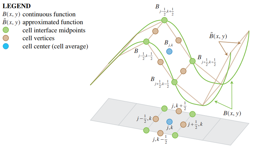
2D linear piecewise reconstruction. Source: Horváth et al. (2014)[2]
Application of reconstructed elevation Source: Horváth et al. (2014)[2]
.PNG)
.PNG)
Notes
- An alternative elevation model can be provided as a prequel.
- The smaller the grid size, the closer the bottom reconstruction will approximate the original surface elevation.
- The resulting elevation model can be inspected in a project using the SURFACE_ELEVATION result type.
References
- ↑ 1.0 1.1 Kurganov A, Petrova G (2007) ∙ A Second-Order Well-Balanced Positivity Preserving Central-Upwind Scheme for the Saint-Venant System ∙ found at: http://www.math.tamu.edu/~gpetrova/KPSV.pdf (last visited 2018-06-29)
- ↑ 2.0 2.1 Zsolt Horváth, Jürgen Waser, Rui A. P. Perdigão, Artem Konev and Günter Blöschl (2014) ∙ A two-dimensional numerical scheme of dry/wet fronts for the Saint-Venant system of shallow water equations ∙ found at: http://citeseerx.ist.psu.edu/viewdoc/download?doi=10.1.1.700.7977&rep=rep1&type=pdf ∙ http://visdom.at/media/pdf/publications/Poster.pdf ∙ (last visited 2018-06-29)


- Models
- Surface • Ground • Rain • Evaporation • Infiltration • Elevation • Breach • Sewer • Storage • Tracer flow • Border • Order
- Model formulas
- Timestep • Season • Surface water level • Groundwater level
- Flow formulas
- Surface flow • Surface infiltration • Ground flow • Ground infiltration • Surface evaporation • Ground evaporation • Ground bottom flow
- Hydraulic structure formulas
- Culvert • Weir • Breach growth • Breach flow • Pump • Sewer Overflow • Inlet • Drainage
- Related