Excel Indicator: Difference between revisions
| (281 intermediate revisions by 9 users not shown) | |||
| Line 1: | Line 1: | ||
{| | The Excel Indicator is an [[Indicators|indicator]] that uses a Microsoft Excel File to perform calculations. Spatial information can be send to an uploaded Excel spreadsheet and score and explanation information is retrieved from the file to be displayed in the project main view. | ||
| | |||
Please note that the full offline version of Microsoft Excel is required and the file format used is the xlsx-format. Also, we can not guarantee that other (open source and online MS Office) packages offer the same functionality as the full offline version of Microsoft Excel, such as the naming of cells and expandable entry fields for longer cell names. | |||
[[File:ExcelFlow2-Q3-2015.jpg|300px|left]] | |||
<br clear=all> | |||
===How is the Excel Indicator implemented in the {{software}}?=== | |||
The {{software}} uses spatial data sets from different sources. If this data set contains information that can be retrieved with a [[TQL|query]], a dedicated indicator in the form of an (xlsx) Excel spreadsheet can be created by the user to process this data. A change in the project state provides input to the indicator, the indicator spreadsheet performs calculations based on this input and displays the result as output in the indicator and progress panel on the top bar.<br /> | |||
[[File:exce10a-Q3-2015.jpg|left|thumb|Detail from sample Indicator Excel File]] | |||
<br clear=all> | |||
To better understand the implementation of the Excel Indicator, please read the [[#Prerequisites|Prerequisites]] and [[#Getting Started (with an example)|Getting Started (with an example)]] sections below. | |||
==Prerequisites== | |||
In order for the Excel indicator to work, the spreadsheet must contain the following: | |||
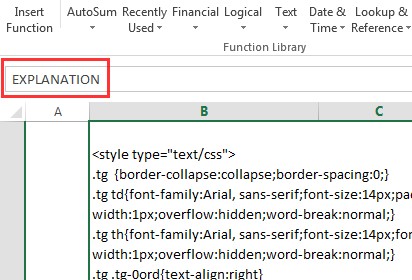
* A cell named <code>EXPLANATION</code>, containing a (html-) text string or table to display the indicator output. | |||
The Explanation Text in the <code>EXPLANATION</code> cell can contain the variables <code>%s</code>, which will be replaced by cells named: | |||
*<code>VAR_0</code> | |||
*<code>VAR_1</code> | |||
*<code>VAR_2</code>, and so on... | |||
If the Explanation Text contains a total of ''n'' <code>%s</code> variables, <code>VAR_0</code> to <code>VAR_(n-1)</code> should be present as named cells. The first <code>%s</code> will be replaced by the output of the cell named <code>VAR_0</code>, the second <code>%s</code> with <code>VAR_1</code>, and the ''n'' <code>%s</code> will thus be replaced with <code>VAR_(n-1)</code>. In other words, an <code>EXPLANATION</code> text containing 10 <code>%s</code> variables, will require cells named from <code>VAR_0</code> to <code>VAR_9</code>. | |||
(Note: to display an actual percentage sign in the explanation, you need to place two percentage signs. I.e. : "50% of houses" should be written as "50%% of houses") | |||
As a rule of thumb, a cell must contain a name and/ or a value. The name can consist of a text string, such as <code>EXPLANATION</code> or <code>SCORE</code>, a variable designation (<code>VAR_#</code>) or a query (<code>SELECT_UNITS_WHERE_CATEGORY_IS_SOCIAL_AND_MAP_IS_CURRENT</code>) in order to load data from the project. Cell values can consist of actual values or text strings, a reference to the value of another cell, or formulas that return a processed value as output. | |||
<gallery> | |||
File:ExcelExplanation-Q3-2015.jpg|<code>EXPLANATION</code> | |||
File:ExcelScoreMaquette-Q3-2015.jpg|<code>SCORE_MAQUETTE</code> | |||
File:ExcelScoreCurrent-Q3-2015.jpg|<code>SCORE_CURRENT</code> | |||
File:ExcelVar_0-Q3-2015.jpg|<code>VAR_0</code> | |||
File:Excel_s_Variable-Q3-2015.jpg|<code>%s</code> variable | |||
File:ExcelNameQuery-Q3-2015.jpg|Query as name | |||
File:ExcelTextValue-Q3-2015.jpg|String as value | |||
File:ExcelFuncValue-Q3-2015.jpg|Formula as value | |||
</gallery> | |||
==Getting Started (with an example)== | |||
This section contains a tutorial on how to create a spreadsheet that will be able to perform as an Excel Indicator in the {{software}}. We will go through this process step-by-step with a use case in Lower Manhattan (New York, USA) as example project, dealing with flood hazard and safe zones. The indicator will score on the amount of housing units protected, both before and after implementing flood protection measures, such as levees and barriers. | |||
: ''A complete Excel Workbook with this example is available to download: http://support.tygron.com/w/downloads/examples/LM_NYC_Housing_TQL_150804-VVD-0.1.xlsx'' | |||
===Example Setup=== | |||
First create a new blank Excel workbook/ spreadsheet. In the image below you can see a spreadsheet with [[Function|Function Categories]]. For the Lower Manhattan use case we are interested in calculating the amount of housing units per building type that are protected within a safe zone. In the {{software}}, a project, situated around Lower Manhattan, containing a Safe Zone [[Areas#Safe zone|Areas]], has already been created. This project is conveniently named "Lower Manhattan". The Safe Zone terrain of this project has been imported from [https://www.arcgis.com/features ArcGIS], based on the National Flood Hazard Layer (NFHL) from the Federal Emergency Agency (FEMA). | |||
<gallery> | |||
File:excel-func-cat-Q3-2015.jpg|Spreadsheet with function categories | |||
File:excel-lower-manhattan-Q3-2015.jpg|Lower Manhattan project with Safe Zone terrain | |||
</gallery> | |||
===Naming Cells=== | |||
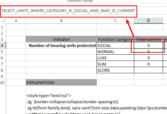
To let the spreadsheet read the amount of housing units within the Safe Zone from the project, a cell must be given a specific name. The name field is shown in the upper left corner of the spreadsheet. The name given in this example is actually a query command that can be interpreted by the {{software}}. Such queries use the [[TQL|Tygron Query Language (TQL)]]. | |||
In this case it says: | |||
<code>SELECT_UNITS_WHERE_CATEGORY_IS_SOCIAL_AND_MAP_IS_MAQUETTE_AND_TERRAINTYPE_IS_SAFE_ZONE</code> | |||
This query is not hard to read or understand;<br /> | |||
<code>Select all units</code> > <code>of the social (affordable) housing category</code> > <code>that are planned</code> > <code>in the protected area</code>. | |||
For another example, to retrieve the total amount of both protected and unprotected Affordable Housing in the area, the query reads as follows: | |||
<code>SELECT_UNITS_WHERE_CATEGORY_IS_SOCIAL_AND_MAP_IS_MAQUETTE</code> | |||
To assist in configuring these queries, a [[Query Tool]] is available in the {{software}} editor. This tool also aids in testing queries. | |||
We start in a cell by creating a column of '''''function categories''''', containing entries for '''''affordable housing (SOCIAL), normal housing (NORMAL), top market housing (LUXE), SUM''''' and '''''SCORE'''''. After this column we add the following columns: '''''Total current, In safe zone current, Unprotected current, In safe zone planned, SZP (In safe zone planned)- SZC (In safe zone current), Total planned, VAR1, VAR2, VAR3, VAR4 and VAR5'''''. | |||
{| class="wikitable" | |||
|- | |||
! scope="col"| Indicator | |||
! scope="col"| Function Category | |||
! scope="col"| Total current | |||
! scope="col"| In safe zone current | |||
! scope="col"| Unprotected Current | |||
! scope="col"| In safe zone planned | |||
! scope="col"| SZP-SZC | |||
! scope="col"| Total Planned | |||
! scope="col"| VAR1 | |||
! scope="col"| VAR2 | |||
! scope="col"| VAR3 | |||
! scope="col"| VAR4 | |||
! scope="col"| VAR5 | |||
|- | |||
! scope="row"| Number of housing units protected | |||
| SOCIAL | |||
| 0 | |||
| 0 | |||
| 0 | |||
| 0 | |||
| 0 | |||
| 0 | |||
| 0 | |||
| 0 | |||
| 0 | |||
| 0 | |||
| 0 | |||
|- | |||
! scope="row"| | |||
| NORMAL | |||
| 0 | |||
| 0 | |||
| 0 | |||
| 0 | |||
| 0 | |||
| 0 | |||
| 0 | |||
| 0 | |||
| 0 | |||
| 0 | |||
| 0 | |||
|- | |||
! scope="row"| | |||
| LUXE | |||
| 0 | |||
| 0 | |||
| 0 | |||
| 0 | |||
| 0 | |||
| 0 | |||
| 0 | |||
| 0 | |||
| 0 | |||
| 0 | |||
| 0 | |||
|- | |||
! scope="row"| | |||
| SUM | |||
| 0 | |||
| 0 | |||
| 0 | |||
| 0 | |||
| 0 | |||
| 0 | |||
| 0 | |||
| 0 | |||
| 0 | |||
| 0 | |||
| 0 | |||
|- | |||
! scope="row"| | |||
| SCORE | |||
| - | |||
| - | |||
| - | |||
| - | |||
| - | |||
| - | |||
| 0 | |||
| 0 | |||
| - | |||
| - | |||
| - | |||
|} | |} | ||
= | ''Please note that all the zero's refer to the default state. The above example is not uploaded to the project yet.'' | ||
The | |||
====Total Current==== | |||
: The cells in this column (Column D in the example file) use the following queries to retrieve the total amount of units present per function category from the project data. Queries are entered in the Name field.<br> | |||
: <code>SELECT_UNITS_WHERE_CATEGORY_IS_SOCIAL_AND_MAP_IS_CURRENT</code><br> | |||
: <code>SELECT_UNITS_WHERE_CATEGORY_IS_NORMAL_AND_MAP_IS_CURRENT</code><br> | |||
: <code>SELECT_UNITS_WHERE_CATEGORY_IS_LUXE_AND_MAP_IS_CURRENT</code><br> | |||
: The <code>SUM</code> cell contains a simple formula adding up the above cells: <code>=SUM(D4;D5;D6)</code><br> | |||
====In safe zone current (SZC)==== | |||
: The cells in this column (Column E in the example file) use the following queries to retrieve the amount of currently protected units per function category from the project data. Queries are entered in the Name field.<br> | |||
: <code>SELECT_UNITS_WHERE_CATEGORY_IS_SOCIAL_AND_MAP_IS_CURRENT_AND_TERRAINTYPE_IS_SAFE_ZONE</code><br> | |||
: <code>SELECT_UNITS_WHERE_CATEGORY_IS_NORMAL_AND_MAP_IS_CURRENT_AND_TERRAINTYPE_IS_SAFE_ZONE</code><br> | |||
: <code>SELECT_UNITS_WHERE_CATEGORY_IS_LUXE_AND_MAP_IS_CURRENT_AND_TERRAINTYPE_IS_SAFE_ZONE</code><br> | |||
: The <code>SUM</code> cell contains a simple formula adding up the above cells: <code>=SUM(E4;E5;E6)</code><br> | |||
====Unprotected Current==== | |||
: The cells in this column (Column F in the example file) use the following formulas to calculate the currently unprotected units per function category. Formulas are entered in the Function field (Fx).<br> | |||
: <code>=SUM(D4;-E4)</code><br> | |||
: <code>=SUM(D5;-E5)</code><br> | |||
: <code>=SUM(D6;-E6)</code><br> | |||
: The <code>SUM</code> cell contains a simple formula adding up the above cells: <code>=SUM(F4;F5;F6)</code><br> | |||
====In safe zone planned (SZP)==== | |||
: The cells in this column (Column G in the example file) use the following queries to retrieve the total amount of units in the planned (= MAQUETTE) Safe Zone, per function category, from the project data. Queries are entered in the Name field.<br> | |||
: <code>SELECT_UNITS_WHERE_CATEGORY_IS_SOCIAL_AND_MAP_IS_MAQUETTE_AND_TERRAINTYPE_IS_SAFE_ZONE</code><br> | |||
: <code>SELECT_UNITS_WHERE_CATEGORY_IS_NORMAL_AND_MAP_IS_MAQUETTE_AND_TERRAINTYPE_IS_SAFE_ZONE</code><br> | |||
: <code>SELECT_UNITS_WHERE_CATEGORY_IS_LUXE_AND_MAP_IS_MAQUETTE_AND_TERRAINTYPE_IS_SAFE_ZONE</code><br> | |||
: The <code>SUM</code> cell contains a simple formula adding up the above cells: <code>=SUM(G4;G5;G6)</code><br> | |||
====SZP (In safe zone planned) minus SZC (In safe zone current)==== | |||
: The cells in this column (Column H in the example file) use the below formulas (Safe Zone Planned minus Safe Zone Current) to calculate the amount of units being added to the planned Safe Zone. Formulas are entered in the Function field (Fx).<br> | |||
: <code>=SUM(G4;-E4)</code><br> | |||
: <code>=SUM(G5;-E5)</code><br> | |||
: <code>=SUM(G6;-E6)</code><br> | |||
: The <code>SUM</code> cell contains a simple formula adding up the above cells: <code>=SUM(H4;H5;H6)</code><br> | |||
====Total Planned==== | |||
: The cells in this column (Column I in the example file) use the following queries to retrieve the total amount of planned units per function category, from the project data. If no new housing units are added to or removed from the project area, this should equal the Total current column. Queries are entered in the Name field.<br> | |||
: <code>SELECT_UNITS_WHERE_CATEGORY_IS_SOCIAL_AND_MAP_IS_MAQUETTE</code><br> | |||
: <code>SELECT_UNITS_WHERE_CATEGORY_IS_NORMAL_AND_MAP_IS_MAQUETTE</code><br> | |||
: <code>SELECT_UNITS_WHERE_CATEGORY_IS_LUXE_AND_MAP_IS_MAQUETTE</code><br> | |||
: The <code>SUM</code> cell contains a simple formula adding up the above cells: <code>=SUM(I4;I5;I6)</code><br> | |||
====VAR1==== | |||
: This column (J in the example file) retrieves the value of the Total Current column and rounds the value up to whole numbers with the following formulas: | |||
: <code>=ROUND(D4;0)</code><br> | |||
: <code>=ROUND(D5;0)</code><br> | |||
: <code>=ROUND(D6;0)</code><br> | |||
: This value can then be retrieved by a variable <code>%s</code> in the <code>EXPLANATION</code>. | |||
The | : The <code>SUM</code> cell contains a formula rounding up the totals of the original cells: <code>=ROUND(D7;0)</code><br> | ||
<code> | ====VAR2==== | ||
: This column (K in the example file) retrieves the value of the In Safe Zone Current column and rounds the value up to whole numbers with the following formulas: | |||
: <code>=ROUND(E4;0)</code><br> | |||
: <code>=ROUND(E5;0)</code><br> | |||
: <code>=ROUND(E6;0)</code><br> | |||
This | : This value can then be retrieved by a variable <code>%s</code> in the <code>EXPLANATION</code>. | ||
<code> | : The <code>SUM</code> cell contains a formula rounding up the totals of the original cells: <code>=ROUND(E7;0)</code><br> | ||
====VAR3==== | |||
: This column (L in the example file) retrieves the value of the SZP (In safe zone planned)- SZC (In safe zone current) column and rounds the value up to whole numbers with the following formulas: | |||
: <code>=ROUND(H4;0)</code><br> | |||
: <code>=ROUND(H5;0)</code><br> | |||
: <code>=ROUND(H6;0)</code><br> | |||
: This value can then be retrieved by a variable <code>%s</code> in the <code>EXPLANATION</code>. | |||
: The <code>SUM</code> cell contains a formula rounding up the totals of the original cells: <code>=ROUND(H7;0)</code><br> | |||
====VAR4==== | |||
: This column (M in the example file) retrieves the value of the In safe zone planned (SZP) column and rounds the value up to whole numbers with the following formulas: | |||
: <code>=ROUND(G4;0)</code><br> | |||
: <code>=ROUND(G5;0)</code><br> | |||
: <code>=ROUND(G6;0)</code><br> | |||
: This value can then be retrieved by a variable <code>%s</code> in the <code>EXPLANATION</code>. | |||
<gallery | : The <code>SUM</code> cell contains a formula rounding up the totals of the original cells: <code>=ROUND(G7;0)</code><br> | ||
====VAR5==== | |||
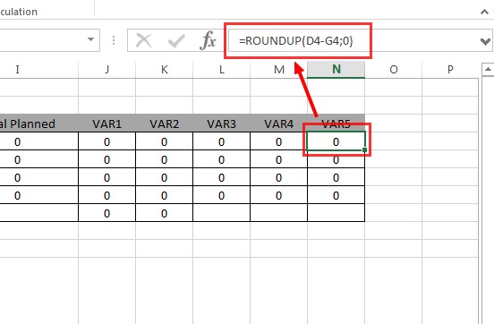
: This column (N in the example file) calculates and rounds up the amount of units that remain unprotected, with the following formulas: | |||
: <code>=ROUNDUP(D4-G4;0)</code><br> | |||
: <code>=ROUNDUP(D5-G5;0)</code><br> | |||
: <code>=ROUNDUP(D6-G6;0)</code><br> | |||
: This value can then be retrieved by a variable <code>%s</code> in the <code>EXPLANATION</code>. | |||
: The <code>SUM</code> cell contains a formula rounding up the totals of the original cells: <code>=ROUNDUP(D7-G7;0)</code><br> | |||
====SCORE==== | |||
: These cells can contain different formulas. In general the score is a percentage of the scoring value on as a fraction of the total value. | |||
: <code>SCORE_CURRENT</code>: <code>=E7/IF(D7;D7;1)</code> = In safe zone current (SZC)/ Total Current (if Total Current > 0, with one decimal significance) | |||
: <code>SCORE_MAQUETTE</code>: <code>=G7/IF(I7;I7;1)</code> = In safe zone planned (SZP)/ Total Plannend (if Total Planned > 0, with one decimal significance) | |||
===Editing Named Cells=== | |||
The naming of cells should be done carefully, because any mistake here will result in an error during the calculation of the Excel Indicator. Once a cell has been labelled with a name, the Microsoft Excel Name Manager must be used to edit or remove the name of the cell. The Name Manager can be opened as follows; select Formulas → Defined Names → Name Manager. | |||
<gallery> | |||
File:ExcelNameManagerRibbon-Q3-2015.jpg|How to open the Excel Name Manager | |||
File:Excel_quick_start_4.jpg|Excel Name Manager panel | |||
</gallery> | </gallery> | ||
In order to generate scores | On the Excel Name Manager panel you can find all defined names in the workbook and to what cells these names refer. If you want to edit a cell name, highlight it and select the Edit Button. The following panel will then appear: | ||
[[File:ExcelNameManagerEdit-Q3-2015.jpg|thumb|left|Edit Cell Name]] | |||
<br clear=all> | |||
To delete a cell name, highlight the entry and select Delete. A message will ask for confirmation. | |||
[[File:ExcelNameManagerDelete-Q3-2015.jpg|thumb|left|Delete Confirmation Message]] | |||
<br clear=all> | |||
You can even select multiple entries at once, by pressing the Shift key when selecting. This can be very convenient when rearranging all VAR_# entries for instance. | |||
[[File:ExcelNameManagerMultiSelect-Q3-2015.jpg|thumb|left]] | |||
<br clear=all> | |||
===Fixing Name Problems=== | |||
In the Name Manager panel you can edit both the name as well as the cell it refers to. This is the easiest way to correct a naming issue. It is possible to (incorrectly) refer two or more labels to the same cell, as the image below shows. In this example both a <code>MAQUETTE</code> and a <code>CURRENT</code> query are referring to the same cell. One will override the other and the order is unpredictable. Please make sure to resolve these issues first. You can delete the name, or let it refer to another cell. | |||
[[File:Excel_quick_start_6a.jpg|thumb|left|600px|Errors in cell naming]] | |||
<br clear=all> | |||
===Indicator Scores=== | |||
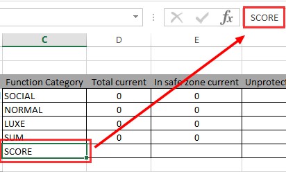
To be able to generate scores from the Excel indicator, there needs to be either one cell named <code>SCORE</code>, or two cells named <code>SCORE_CURRENT</code> and <code>SCORE_MAQUETTE</code>. The <code>SCORE_MAQUETTE</code> and <code>SCORE_CURRENT</code> queries can be used to indicate the difference between the planned outcome and the original (current) situation. | |||
<br /> | |||
[[File:ExcelScorePlanned-Q3-2015.jpg|thumb|left|<code>SCORE</code> output]] | |||
<br clear=all> | |||
===Explanation=== | |||
Last but not least is the explanation. This is the text shown in the lower left corner of the Indicator panel during a session. The explanation text can be written in html format. The cell should be named <code>EXPLANATION</code>. When using explanation texts, you may also want to include numbers and/ or text output from your excel. For this you can include <code>%s</code> values, which will be replaced by <code>VAR_#</code> cells, starting from <code>VAR_0</code>. See also [[#Prerequisites|Prerequisites]]. | |||
[[File:ExcelIndicatorPanelExplanation2-Q3-2015.jpg|thumb|left|Explanation field on Indicator Panel]] | |||
<br clear=all> | |||
====Simple text string as EXPLANATION output==== | |||
A simple HTML text string as <code>EXPLANATION</code> output can be written as follows: | |||
<code><nowiki><p>SOCIAL:%s units total, of which %s are currently protected, %s are planned to be protected, protecting a total of %s units, leaving %s units unprotected</p></nowiki></code> | |||
In this string, values from cells named <code>VAR_0</code> to <code>VAR_4</code> are being used to output values in the explanation text. | |||
Combining three strings with only a change in category names will cover <code>VAR_0</code> to <code>VAR_18</code> and results in the following: | |||
<code><nowiki><p>SOCIAL:%s units total, of which %s are currently protected, %s are planned to be protected, protecting a total of %s units, leaving %s units unprotected</p></nowiki></code><br/> | |||
<code><nowiki><p>NORMAL:%s units total, of which %s are currently protected, %s are planned to be protected, protecting a total of %s units, leaving %s units unprotected</p></nowiki></code><br/> | |||
<code><nowiki><p>LUXE:%s units total, of which %s are currently protected, %s are planned to be protected, protecting a total of %s units, leaving %s units unprotected</p></nowiki></code><br/> | |||
==Tips== | Which looks on the Excel Indicator panel in the project main view like this: | ||
*Divisions by zero can be solved as | |||
[[File:ExcelIndicatorTextlExplanation-Q3-2015.jpg|thumb|left|Text string as <code>EXPLANATION</code>]] | |||
<br clear=all> | |||
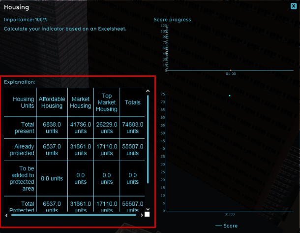
====HTML table as EXPLANATION output==== | |||
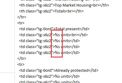
As the above shows, with many <code>VAR_#</code> variables and categories present, the <code>EXPLANATION</code> field tends to lack clarity. To improve readability of the <code>EXPLANATION</code> output, it is recommended to implement a table format. This can be done by using personal HTML skills, however, as this can be a bit too advanced for general users, we recommend using an HTML table generator, such as: http://www.tablesgenerator.com/html_tables#. | |||
Following steps on this page will result in an HTML based table that can be copied onto the EXPLANATION cell in the spreadsheet and then loaded into the {{software}}. | |||
Such a table will look like this in HTML: | |||
<code><nowiki>"<style type=""text/css""> | |||
.tg {border-collapse:collapse;border-spacing:0;} | |||
.tg td{font-family:Arial, sans-serif;font-size:14px;padding:10px 5px;border-style:solid;border-width:1px;overflow:hidden;word-break:normal;} | |||
.tg th{font-family:Arial, sans-serif;font-size:14px;font-weight:normal;padding:10px 5px;border-style:solid;border-width:1px;overflow:hidden;word-break:normal;} | |||
.tg .tg-0ord{text-align:right} | |||
.tg .tg-s6z2{text-align:center} | |||
</style> | |||
<table class=""tg""> | |||
<tr> | |||
<th class=""tg-0ord"">Housing Units</th> | |||
<th class=""tg-s6z2"">Affordable Housing<br></th> | |||
<th class=""tg-s6z2"">Market Housing<br></th> | |||
<th class=""tg-s6z2"">Top Market Housing<br></th> | |||
<th class=""tg-s6z2"">Totals<br></th> | |||
</tr> | |||
<tr> | |||
<td class=""tg-0ord"">Total present</td> | |||
<td class=""tg-s6z2"">%s units<br></td> | |||
<td class=""tg-s6z2"">%s units</td> | |||
<td class=""tg-s6z2"">%s units</td> | |||
<td class=""tg-s6z2"">%s units</td> | |||
</tr> | |||
<tr> | |||
<td class=""tg-0ord"">Already protected</td> | |||
<td class=""tg-s6z2"">%s units</td> | |||
<td class=""tg-s6z2"">%s units</td> | |||
<td class=""tg-s6z2"">%s units</td> | |||
<td class=""tg-s6z2"">%s units</td> | |||
</tr> | |||
<tr> | |||
<td class=""tg-0ord"">To be added to protected area</td> | |||
<td class=""tg-s6z2"">%s units</td> | |||
<td class=""tg-s6z2"">%s units</td> | |||
<td class=""tg-s6z2"">%s units</td> | |||
<td class=""tg-s6z2"">%s units</td> | |||
</tr> | |||
<tr> | |||
<td class=""tg-0ord"">Total Protected<br></td> | |||
<td class=""tg-s6z2"">%s units</td> | |||
<td class=""tg-s6z2"">%s units</td> | |||
<td class=""tg-s6z2"">%s units</td> | |||
<td class=""tg-s6z2"">%s units</td> | |||
</tr> | |||
<tr> | |||
<td class=""tg-0ord"">Remaining unprotected</td> | |||
<td class=""tg-s6z2"">%s units</td> | |||
<td class=""tg-s6z2"">%s units</td> | |||
<td class=""tg-s6z2"">%s units</td> | |||
<td class=""tg-s6z2"">%s units</td> | |||
</tr> | |||
</table>" | |||
</nowiki></code> | |||
This will result in the following table: | |||
{| class="wikitable" | |||
|- | |||
! scope="col"| Housing Units | |||
! scope="col"| Affordable Housing | |||
! scope="col"| Market Housing | |||
! scope="col"| Top Market Housing | |||
! scope="col"| Totals | |||
|- | |||
! scope="row"| Total present | |||
| %s units | |||
| %s units | |||
| %s units | |||
| %s units | |||
|- | |||
! scope="row"| Already protected | |||
| %s units | |||
| %s units | |||
| %s units | |||
| %s units | |||
|- | |||
! scope="row"| To be added to protected area | |||
| %s units | |||
| %s units | |||
| %s units | |||
| %s units | |||
|- | |||
! scope="row"| Total Protected | |||
| %s units | |||
| %s units | |||
| %s units | |||
| %s units | |||
|- | |||
! scope="row"| Remaining unprotected | |||
| %s units | |||
| %s units | |||
| %s units | |||
| %s units | |||
|} | |||
[[File:ExcelTableExplanation-Q3-2015.jpg|thumb|left|HTML table as <code>EXPLANATION</code>]] | |||
<br clear=all> | |||
===Exact=== | |||
: The following output labels can be used to show text or numbers in the indicator panel at the top bar. | |||
: <code>EXACT_NUMBER_VALUE</code>: A numerical value that is formatted using the unit system selected for your project. Replaces the indicator's progress bar. | |||
: <code>EXACT_NUMBER_VALUE_CURRENT</code>: A numerical value for the current situation that is formatted using the unit system selected for your project. Replaces the indicator's progress bar. | |||
: <code>EXACT_NUMBER_VALUE_MAQUETTE</code>: A numerical value for the maquette situation that is formatted using the unit system selected for your project. Replaces the indicator's progress bar. | |||
: <code>EXACT_TEXT_VALUE</code>: A text value that will be used instead of the progress bar. | |||
: <code>EXACT_TEXT_VALUE_CURRENT</code>: A text value for the current situation that will be used instead of the progress bar. | |||
: <code>EXACT_TEXT_VALUE_MAQUETTE</code>: A text value for the maquette situation that will be used instead of the progress bar. | |||
==Upload an Excel file== | |||
To upload an Excel xlsx-file for the Excel Indicator, have the file ready on an easy to remember location (desktop for instance), and add in the Editor an Excel indicator to the project. Select Excel File Name on the left panel and select the Upload button on the right panel. In the newly opened panel, select the file to upload and confirm. Now the file has been uploaded to the project, and the new indicator has appeared on the top bar. If there was already a previous version of the file present, please select the [[calculation_panel|Recalculate Indicators]] option from the Indicators drop down menu, to ensure the newly uploaded spreadsheet has an actual impact on the project. | |||
<br> | |||
<br> | |||
{{Editor steps|title=upload an Excel Indicator|Select Indicators > Add Excel Indicator|Rename the newly added indicator in the 'Name' and Short Name' fields on the right panel|Select the color to be used in the progression panel|Select to activate the indicator, if desired|Add a proper description|Highlight 'Excel File Name' on the left panel panel|Select the 'Upload' button|Select the file to upload in the 'Choose your file' panel|Select Indicators > recalculate Indicators}} | |||
<br clear=all> | |||
<gallery mode=nolines> | |||
File:AddExcelIndicator-Q3-2015.jpg|1. Select Indicators > Indicators > Add Excel Indicator | |||
File:RenameExcelIndicator-Q3-2015.jpg|2. Enter new Name and Short Name | |||
File:ChangeColorExcelIndicator-Q3-2015.jpg|3. Change color of the indicator | |||
File:ActivateExcelIndicator-Q3-2015.jpg|4. Activate the indicator | |||
File:AddDescriptionExcelIndicator-Q3-2015.jpg|5. Add a description | |||
File:HighlightExcelFileName-Q3-2015.jpg|6. Highlight 'Excel File Name' on the left panel | |||
File:SelectUploadExcelIndicator-Q3-2015.jpg|7. Select the 'Upload' button | |||
File:SelectFileExcelIndicator-Q3-2015.jpg|8. Select the file to upload in the 'Choose your file' panel | |||
File:RecalculateExcelIndicator-Q3-2015.jpg|9. Recalculate the newly added Excel indicator | |||
</gallery> | |||
==Summary (how to...)== | |||
: Below is a small summary describing a suggested workflow from a bird's eye perspective, without going deeper into details: | |||
<br> | |||
{{Editor steps|title=create an Excel Indicator|Load the sample project Lower Manhattan in the editor.|Create an empty xlsx workbook.|Name one cell <code>EXPLANATION</code>.|Create the <code>EXPLANATION</code> output format (HTML text string, HTML table) with <code>%s</code> variables.|Decide, based on the <code>EXPLANATION</code>, which function categories are needed, and place them in one column.|Add consecutive columns that match the <code>EXPLANATION</code>.|Create the <code>VAR</code> columns with <code>ROUND(UP)</code> formulas and <code>VAR_n</code> name labels.|Create the <code>SCORE</code> field(s) as required by the type of project (Timeline/ Planning).|Optionally, test the spreadsheet by entering round values in query fields.|Create a new Excel Indicator in the project and upload the Excel file to the project.|Recalculate the indicators and verify if no errors are present.}} | |||
===Tips=== | |||
*Divisions by zero can be solved as follows: <code>=C2/IF(D2,D2,1)</code>. In this example cells C2 and D2 contain number values. | |||
*Instead of using the VAR_# method for the explanation text, you can also use the concatenate function of excel: | *Instead of using the VAR_# method for the explanation text, you can also use the concatenate function of excel: | ||
<code>CONCATENATE( | <code> | ||
CONCATENATE(<nowiki>"<p>",A2, ": ", E2, " m2 and in Safe Zone: ", F2, " m2</p>"</nowiki>) | |||
</code> | |||
*Starting with creating a table aids in setting up the Excel spreadsheet, by already thinking in advance about the lay out and formatting of the <code>EXPLANATION</code>. | |||
*To quickly test the spreadsheet, without uploading it to the project, it is possible to enter some values in all the cells that contain queries as name. Other cells with formulas will change their content accordingly. By entering round values, for example 100, 1000, etc, calculations can easily be verified. Don't forget to save first and to revert back to the last saved version when done verifying! | |||
*To display an actual percentage sign in the explanation, you need to place two percentage signs. I.e. : "50% of houses" should be written as "50%% of houses". | |||
==Extras== | |||
: As practice on these Excel indicators, try to create the following indicators for Lower Manhattan: | |||
:*Create an Excel indicator for protected floor sizes instead of for protected units of different categories. | |||
:*Create an Excel indicator for protected floor sizes of Industry, Offices and Commercial buildings. | |||
:*Create an Excel indicator for the amount of jobs being protected. Use for this the following constant values: Industry - 250sq ft/ job, Offices - 50sq ft/job and Commercial - 65sq ft/job. | |||
{{article end | |||
|seealso= | |||
* [[Excel]] | |||
* [[Indicator]] | |||
* [[TQL]] | |||
|howtos= | |||
*[[How to configure a Query for an Excel Indicator]] | |||
*[[How to create an Excel background calculation model]] | |||
*[[How to implement an Excel Indicator]] | |||
*[[How to manually adjust Indicators in Excel]] | |||
*[[How to use the Query Tool to test queries from an Excel Indicator spreadsheet]] | |||
}}{{Indicator nav}} | |||
[[Category:TQL]][[Category:How-to's]][[Category:Indicator]] | |||
Latest revision as of 11:54, 9 October 2023
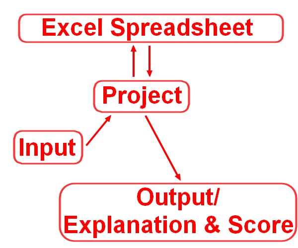
The Excel Indicator is an indicator that uses a Microsoft Excel File to perform calculations. Spatial information can be send to an uploaded Excel spreadsheet and score and explanation information is retrieved from the file to be displayed in the project main view.
Please note that the full offline version of Microsoft Excel is required and the file format used is the xlsx-format. Also, we can not guarantee that other (open source and online MS Office) packages offer the same functionality as the full offline version of Microsoft Excel, such as the naming of cells and expandable entry fields for longer cell names.
How is the Excel Indicator implemented in the Tygron Platform?
The Tygron Platform uses spatial data sets from different sources. If this data set contains information that can be retrieved with a query, a dedicated indicator in the form of an (xlsx) Excel spreadsheet can be created by the user to process this data. A change in the project state provides input to the indicator, the indicator spreadsheet performs calculations based on this input and displays the result as output in the indicator and progress panel on the top bar.
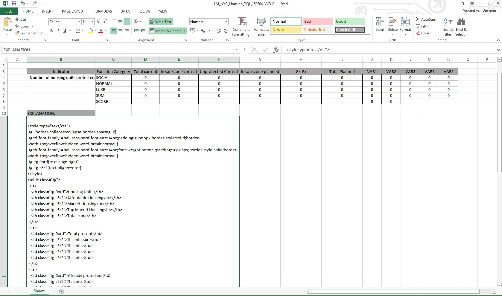
To better understand the implementation of the Excel Indicator, please read the Prerequisites and Getting Started (with an example) sections below.
Prerequisites
In order for the Excel indicator to work, the spreadsheet must contain the following:
- A cell named
EXPLANATION, containing a (html-) text string or table to display the indicator output.
The Explanation Text in the EXPLANATION cell can contain the variables %s, which will be replaced by cells named:
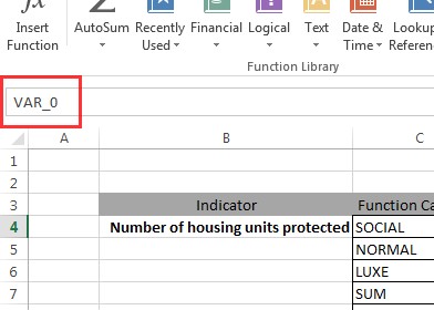
VAR_0VAR_1VAR_2, and so on...
If the Explanation Text contains a total of n %s variables, VAR_0 to VAR_(n-1) should be present as named cells. The first %s will be replaced by the output of the cell named VAR_0, the second %s with VAR_1, and the n %s will thus be replaced with VAR_(n-1). In other words, an EXPLANATION text containing 10 %s variables, will require cells named from VAR_0 to VAR_9.
(Note: to display an actual percentage sign in the explanation, you need to place two percentage signs. I.e. : "50% of houses" should be written as "50%% of houses")
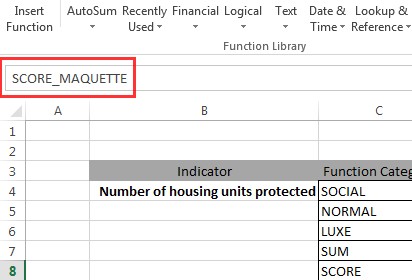
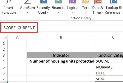
As a rule of thumb, a cell must contain a name and/ or a value. The name can consist of a text string, such as EXPLANATION or SCORE, a variable designation (VAR_#) or a query (SELECT_UNITS_WHERE_CATEGORY_IS_SOCIAL_AND_MAP_IS_CURRENT) in order to load data from the project. Cell values can consist of actual values or text strings, a reference to the value of another cell, or formulas that return a processed value as output.
-
EXPLANATION -
SCORE_MAQUETTE -
SCORE_CURRENT -
VAR_0 -
%svariable -
Query as name
-
String as value
-
Formula as value
Getting Started (with an example)
This section contains a tutorial on how to create a spreadsheet that will be able to perform as an Excel Indicator in the Tygron Platform. We will go through this process step-by-step with a use case in Lower Manhattan (New York, USA) as example project, dealing with flood hazard and safe zones. The indicator will score on the amount of housing units protected, both before and after implementing flood protection measures, such as levees and barriers.
- A complete Excel Workbook with this example is available to download: http://support.tygron.com/w/downloads/examples/LM_NYC_Housing_TQL_150804-VVD-0.1.xlsx
Example Setup
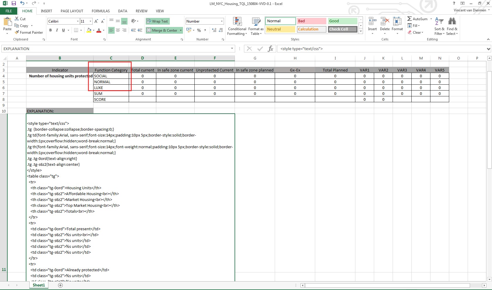
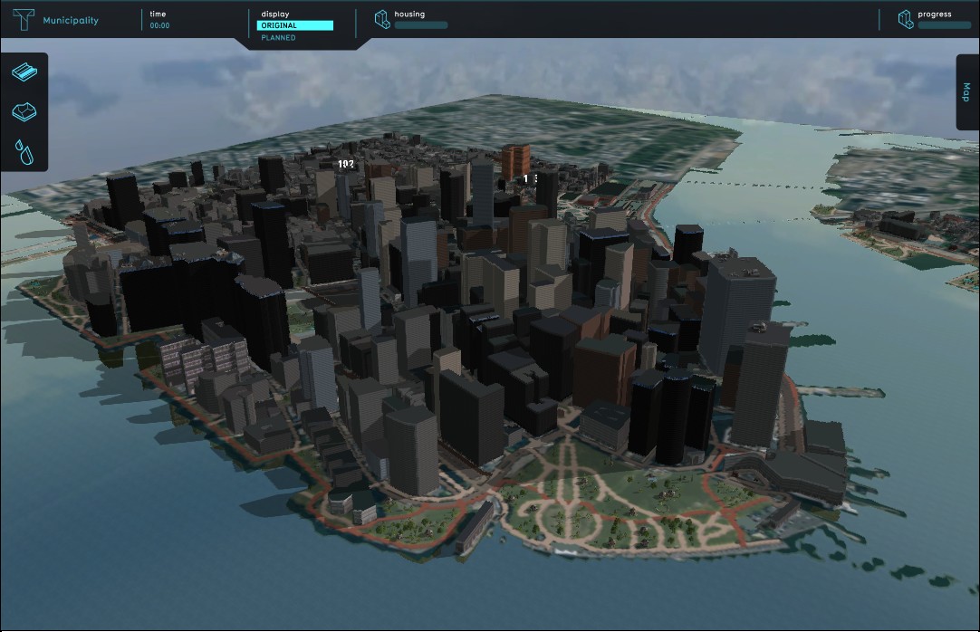
First create a new blank Excel workbook/ spreadsheet. In the image below you can see a spreadsheet with Function Categories. For the Lower Manhattan use case we are interested in calculating the amount of housing units per building type that are protected within a safe zone. In the Tygron Platform, a project, situated around Lower Manhattan, containing a Safe Zone Areas, has already been created. This project is conveniently named "Lower Manhattan". The Safe Zone terrain of this project has been imported from ArcGIS, based on the National Flood Hazard Layer (NFHL) from the Federal Emergency Agency (FEMA).
-
Spreadsheet with function categories
-
Lower Manhattan project with Safe Zone terrain
Naming Cells
To let the spreadsheet read the amount of housing units within the Safe Zone from the project, a cell must be given a specific name. The name field is shown in the upper left corner of the spreadsheet. The name given in this example is actually a query command that can be interpreted by the Tygron Platform. Such queries use the Tygron Query Language (TQL).
In this case it says:
SELECT_UNITS_WHERE_CATEGORY_IS_SOCIAL_AND_MAP_IS_MAQUETTE_AND_TERRAINTYPE_IS_SAFE_ZONE
This query is not hard to read or understand;
Select all units > of the social (affordable) housing category > that are planned > in the protected area.
For another example, to retrieve the total amount of both protected and unprotected Affordable Housing in the area, the query reads as follows:
SELECT_UNITS_WHERE_CATEGORY_IS_SOCIAL_AND_MAP_IS_MAQUETTE
To assist in configuring these queries, a Query Tool is available in the Tygron Platform editor. This tool also aids in testing queries.
We start in a cell by creating a column of function categories, containing entries for affordable housing (SOCIAL), normal housing (NORMAL), top market housing (LUXE), SUM and SCORE. After this column we add the following columns: Total current, In safe zone current, Unprotected current, In safe zone planned, SZP (In safe zone planned)- SZC (In safe zone current), Total planned, VAR1, VAR2, VAR3, VAR4 and VAR5.
| Indicator | Function Category | Total current | In safe zone current | Unprotected Current | In safe zone planned | SZP-SZC | Total Planned | VAR1 | VAR2 | VAR3 | VAR4 | VAR5 |
|---|---|---|---|---|---|---|---|---|---|---|---|---|
| Number of housing units protected | SOCIAL | 0 | 0 | 0 | 0 | 0 | 0 | 0 | 0 | 0 | 0 | 0 |
| NORMAL | 0 | 0 | 0 | 0 | 0 | 0 | 0 | 0 | 0 | 0 | 0 | |
| LUXE | 0 | 0 | 0 | 0 | 0 | 0 | 0 | 0 | 0 | 0 | 0 | |
| SUM | 0 | 0 | 0 | 0 | 0 | 0 | 0 | 0 | 0 | 0 | 0 | |
| SCORE | - | - | - | - | - | - | 0 | 0 | - | - | - |
Please note that all the zero's refer to the default state. The above example is not uploaded to the project yet.
Total Current
- The cells in this column (Column D in the example file) use the following queries to retrieve the total amount of units present per function category from the project data. Queries are entered in the Name field.
SELECT_UNITS_WHERE_CATEGORY_IS_SOCIAL_AND_MAP_IS_CURRENTSELECT_UNITS_WHERE_CATEGORY_IS_NORMAL_AND_MAP_IS_CURRENTSELECT_UNITS_WHERE_CATEGORY_IS_LUXE_AND_MAP_IS_CURRENT
- The
SUMcell contains a simple formula adding up the above cells:=SUM(D4;D5;D6)
In safe zone current (SZC)
- The cells in this column (Column E in the example file) use the following queries to retrieve the amount of currently protected units per function category from the project data. Queries are entered in the Name field.
SELECT_UNITS_WHERE_CATEGORY_IS_SOCIAL_AND_MAP_IS_CURRENT_AND_TERRAINTYPE_IS_SAFE_ZONESELECT_UNITS_WHERE_CATEGORY_IS_NORMAL_AND_MAP_IS_CURRENT_AND_TERRAINTYPE_IS_SAFE_ZONESELECT_UNITS_WHERE_CATEGORY_IS_LUXE_AND_MAP_IS_CURRENT_AND_TERRAINTYPE_IS_SAFE_ZONE
- The
SUMcell contains a simple formula adding up the above cells:=SUM(E4;E5;E6)
Unprotected Current
- The cells in this column (Column F in the example file) use the following formulas to calculate the currently unprotected units per function category. Formulas are entered in the Function field (Fx).
=SUM(D4;-E4)=SUM(D5;-E5)=SUM(D6;-E6)
- The
SUMcell contains a simple formula adding up the above cells:=SUM(F4;F5;F6)
In safe zone planned (SZP)
- The cells in this column (Column G in the example file) use the following queries to retrieve the total amount of units in the planned (= MAQUETTE) Safe Zone, per function category, from the project data. Queries are entered in the Name field.
SELECT_UNITS_WHERE_CATEGORY_IS_SOCIAL_AND_MAP_IS_MAQUETTE_AND_TERRAINTYPE_IS_SAFE_ZONESELECT_UNITS_WHERE_CATEGORY_IS_NORMAL_AND_MAP_IS_MAQUETTE_AND_TERRAINTYPE_IS_SAFE_ZONESELECT_UNITS_WHERE_CATEGORY_IS_LUXE_AND_MAP_IS_MAQUETTE_AND_TERRAINTYPE_IS_SAFE_ZONE
- The
SUMcell contains a simple formula adding up the above cells:=SUM(G4;G5;G6)
SZP (In safe zone planned) minus SZC (In safe zone current)
- The cells in this column (Column H in the example file) use the below formulas (Safe Zone Planned minus Safe Zone Current) to calculate the amount of units being added to the planned Safe Zone. Formulas are entered in the Function field (Fx).
=SUM(G4;-E4)=SUM(G5;-E5)=SUM(G6;-E6)
- The
SUMcell contains a simple formula adding up the above cells:=SUM(H4;H5;H6)
Total Planned
- The cells in this column (Column I in the example file) use the following queries to retrieve the total amount of planned units per function category, from the project data. If no new housing units are added to or removed from the project area, this should equal the Total current column. Queries are entered in the Name field.
SELECT_UNITS_WHERE_CATEGORY_IS_SOCIAL_AND_MAP_IS_MAQUETTESELECT_UNITS_WHERE_CATEGORY_IS_NORMAL_AND_MAP_IS_MAQUETTESELECT_UNITS_WHERE_CATEGORY_IS_LUXE_AND_MAP_IS_MAQUETTE
- The
SUMcell contains a simple formula adding up the above cells:=SUM(I4;I5;I6)
VAR1
- This column (J in the example file) retrieves the value of the Total Current column and rounds the value up to whole numbers with the following formulas:
=ROUND(D4;0)=ROUND(D5;0)=ROUND(D6;0)
- This value can then be retrieved by a variable
%sin theEXPLANATION.
- The
SUMcell contains a formula rounding up the totals of the original cells:=ROUND(D7;0)
VAR2
- This column (K in the example file) retrieves the value of the In Safe Zone Current column and rounds the value up to whole numbers with the following formulas:
=ROUND(E4;0)=ROUND(E5;0)=ROUND(E6;0)
- This value can then be retrieved by a variable
%sin theEXPLANATION.
- The
SUMcell contains a formula rounding up the totals of the original cells:=ROUND(E7;0)
VAR3
- This column (L in the example file) retrieves the value of the SZP (In safe zone planned)- SZC (In safe zone current) column and rounds the value up to whole numbers with the following formulas:
=ROUND(H4;0)=ROUND(H5;0)=ROUND(H6;0)
- This value can then be retrieved by a variable
%sin theEXPLANATION.
- The
SUMcell contains a formula rounding up the totals of the original cells:=ROUND(H7;0)
VAR4
- This column (M in the example file) retrieves the value of the In safe zone planned (SZP) column and rounds the value up to whole numbers with the following formulas:
=ROUND(G4;0)=ROUND(G5;0)=ROUND(G6;0)
- This value can then be retrieved by a variable
%sin theEXPLANATION.
- The
SUMcell contains a formula rounding up the totals of the original cells:=ROUND(G7;0)
VAR5
- This column (N in the example file) calculates and rounds up the amount of units that remain unprotected, with the following formulas:
=ROUNDUP(D4-G4;0)=ROUNDUP(D5-G5;0)=ROUNDUP(D6-G6;0)
- This value can then be retrieved by a variable
%sin theEXPLANATION.
- The
SUMcell contains a formula rounding up the totals of the original cells:=ROUNDUP(D7-G7;0)
SCORE
- These cells can contain different formulas. In general the score is a percentage of the scoring value on as a fraction of the total value.
SCORE_CURRENT:=E7/IF(D7;D7;1)= In safe zone current (SZC)/ Total Current (if Total Current > 0, with one decimal significance)SCORE_MAQUETTE:=G7/IF(I7;I7;1)= In safe zone planned (SZP)/ Total Plannend (if Total Planned > 0, with one decimal significance)
Editing Named Cells
The naming of cells should be done carefully, because any mistake here will result in an error during the calculation of the Excel Indicator. Once a cell has been labelled with a name, the Microsoft Excel Name Manager must be used to edit or remove the name of the cell. The Name Manager can be opened as follows; select Formulas → Defined Names → Name Manager.
-
How to open the Excel Name Manager
-
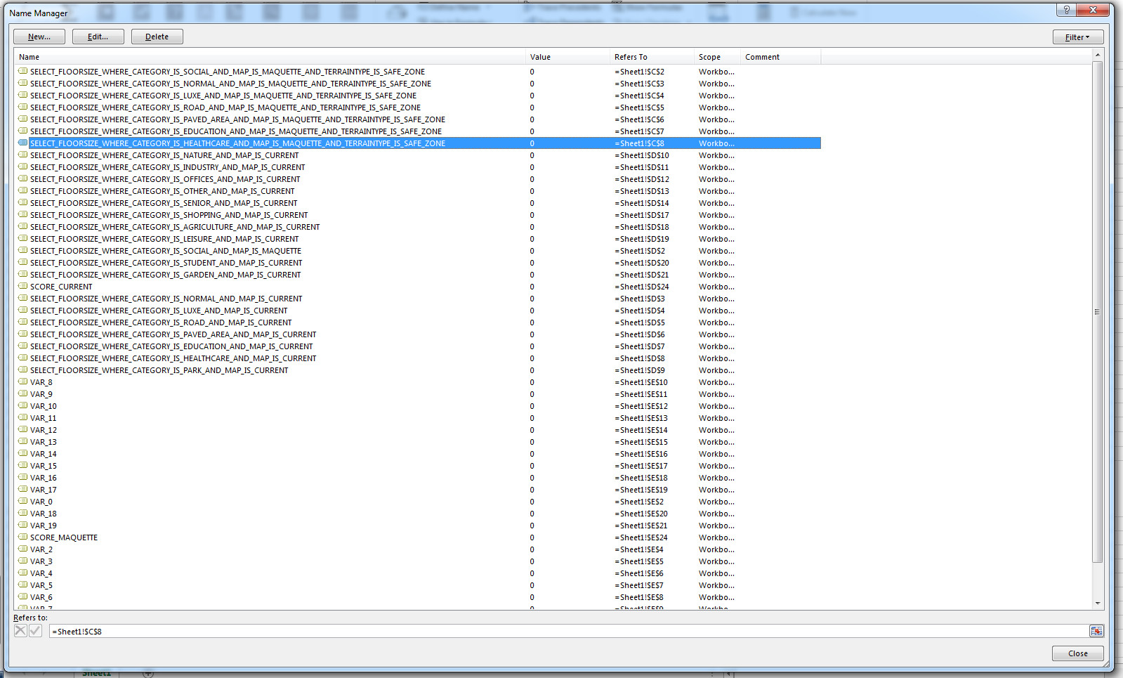
Excel Name Manager panel
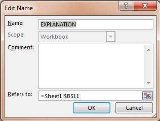
On the Excel Name Manager panel you can find all defined names in the workbook and to what cells these names refer. If you want to edit a cell name, highlight it and select the Edit Button. The following panel will then appear:
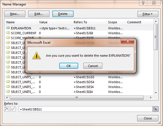
To delete a cell name, highlight the entry and select Delete. A message will ask for confirmation.
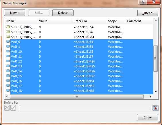
You can even select multiple entries at once, by pressing the Shift key when selecting. This can be very convenient when rearranging all VAR_# entries for instance.
Fixing Name Problems
In the Name Manager panel you can edit both the name as well as the cell it refers to. This is the easiest way to correct a naming issue. It is possible to (incorrectly) refer two or more labels to the same cell, as the image below shows. In this example both a MAQUETTE and a CURRENT query are referring to the same cell. One will override the other and the order is unpredictable. Please make sure to resolve these issues first. You can delete the name, or let it refer to another cell.

Indicator Scores
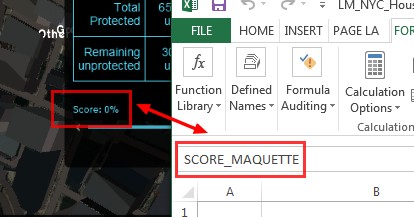
To be able to generate scores from the Excel indicator, there needs to be either one cell named SCORE, or two cells named SCORE_CURRENT and SCORE_MAQUETTE. The SCORE_MAQUETTE and SCORE_CURRENT queries can be used to indicate the difference between the planned outcome and the original (current) situation.
SCORE output
Explanation
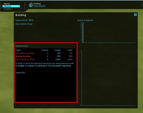
Last but not least is the explanation. This is the text shown in the lower left corner of the Indicator panel during a session. The explanation text can be written in html format. The cell should be named EXPLANATION. When using explanation texts, you may also want to include numbers and/ or text output from your excel. For this you can include %s values, which will be replaced by VAR_# cells, starting from VAR_0. See also Prerequisites.
Simple text string as EXPLANATION output
A simple HTML text string as EXPLANATION output can be written as follows:
<p>SOCIAL:%s units total, of which %s are currently protected, %s are planned to be protected, protecting a total of %s units, leaving %s units unprotected</p>
In this string, values from cells named VAR_0 to VAR_4 are being used to output values in the explanation text.
Combining three strings with only a change in category names will cover VAR_0 to VAR_18 and results in the following:
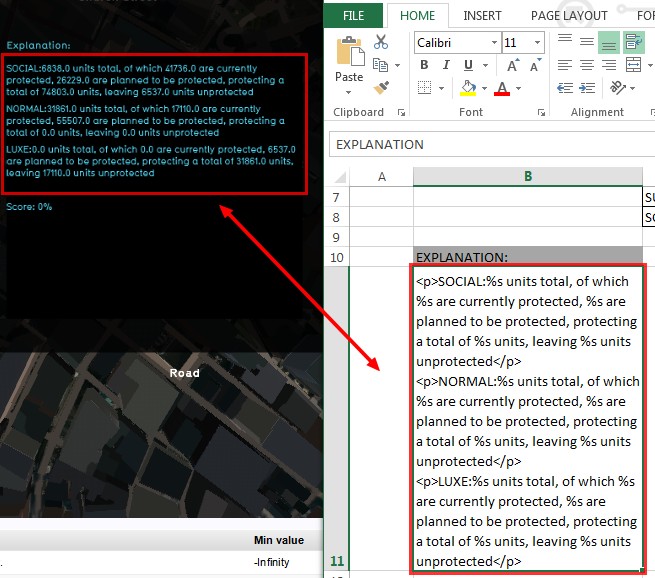
<p>SOCIAL:%s units total, of which %s are currently protected, %s are planned to be protected, protecting a total of %s units, leaving %s units unprotected</p>
<p>NORMAL:%s units total, of which %s are currently protected, %s are planned to be protected, protecting a total of %s units, leaving %s units unprotected</p>
<p>LUXE:%s units total, of which %s are currently protected, %s are planned to be protected, protecting a total of %s units, leaving %s units unprotected</p>
Which looks on the Excel Indicator panel in the project main view like this:
EXPLANATION
HTML table as EXPLANATION output
As the above shows, with many VAR_# variables and categories present, the EXPLANATION field tends to lack clarity. To improve readability of the EXPLANATION output, it is recommended to implement a table format. This can be done by using personal HTML skills, however, as this can be a bit too advanced for general users, we recommend using an HTML table generator, such as: http://www.tablesgenerator.com/html_tables#.
Following steps on this page will result in an HTML based table that can be copied onto the EXPLANATION cell in the spreadsheet and then loaded into the Tygron Platform.
Such a table will look like this in HTML:
"<style type=""text/css"">
.tg  {border-collapse:collapse;border-spacing:0;}
.tg td{font-family:Arial, sans-serif;font-size:14px;padding:10px 5px;border-style:solid;border-width:1px;overflow:hidden;word-break:normal;}
.tg th{font-family:Arial, sans-serif;font-size:14px;font-weight:normal;padding:10px 5px;border-style:solid;border-width:1px;overflow:hidden;word-break:normal;}
.tg .tg-0ord{text-align:right}
.tg .tg-s6z2{text-align:center}
</style>
<table class=""tg"">
  <tr>
    <th class=""tg-0ord"">Housing Units</th>
    <th class=""tg-s6z2"">Affordable Housing<br></th>
    <th class=""tg-s6z2"">Market Housing<br></th>
    <th class=""tg-s6z2"">Top Market Housing<br></th>
    <th class=""tg-s6z2"">Totals<br></th>
  </tr>
  <tr>
    <td class=""tg-0ord"">Total present</td>
    <td class=""tg-s6z2"">%s units<br></td>
    <td class=""tg-s6z2"">%s units</td>
    <td class=""tg-s6z2"">%s units</td>
    <td class=""tg-s6z2"">%s units</td>
  </tr>
  <tr>
    <td class=""tg-0ord"">Already protected</td>
    <td class=""tg-s6z2"">%s units</td>
    <td class=""tg-s6z2"">%s units</td>
    <td class=""tg-s6z2"">%s units</td>
    <td class=""tg-s6z2"">%s units</td>
  </tr>
  <tr>
    <td class=""tg-0ord"">To be added to protected area</td>
    <td class=""tg-s6z2"">%s units</td>
    <td class=""tg-s6z2"">%s units</td>
    <td class=""tg-s6z2"">%s units</td>
    <td class=""tg-s6z2"">%s units</td>
  </tr>
  <tr>
    <td class=""tg-0ord"">Total Protected<br></td>
    <td class=""tg-s6z2"">%s units</td>
    <td class=""tg-s6z2"">%s units</td>
    <td class=""tg-s6z2"">%s units</td>
    <td class=""tg-s6z2"">%s units</td>
  </tr>
  <tr>
    <td class=""tg-0ord"">Remaining unprotected</td>
    <td class=""tg-s6z2"">%s units</td>
    <td class=""tg-s6z2"">%s units</td>
    <td class=""tg-s6z2"">%s units</td>
    <td class=""tg-s6z2"">%s units</td>
  </tr>
</table>"
This will result in the following table:
| Housing Units | Affordable Housing | Market Housing | Top Market Housing | Totals |
|---|---|---|---|---|
| Total present | %s units | %s units | %s units | %s units |
| Already protected | %s units | %s units | %s units | %s units |
| To be added to protected area | %s units | %s units | %s units | %s units |
| Total Protected | %s units | %s units | %s units | %s units |
| Remaining unprotected | %s units | %s units | %s units | %s units |
EXPLANATION
Exact
- The following output labels can be used to show text or numbers in the indicator panel at the top bar.
EXACT_NUMBER_VALUE: A numerical value that is formatted using the unit system selected for your project. Replaces the indicator's progress bar.EXACT_NUMBER_VALUE_CURRENT: A numerical value for the current situation that is formatted using the unit system selected for your project. Replaces the indicator's progress bar.EXACT_NUMBER_VALUE_MAQUETTE: A numerical value for the maquette situation that is formatted using the unit system selected for your project. Replaces the indicator's progress bar.EXACT_TEXT_VALUE: A text value that will be used instead of the progress bar.EXACT_TEXT_VALUE_CURRENT: A text value for the current situation that will be used instead of the progress bar.EXACT_TEXT_VALUE_MAQUETTE: A text value for the maquette situation that will be used instead of the progress bar.
Upload an Excel file
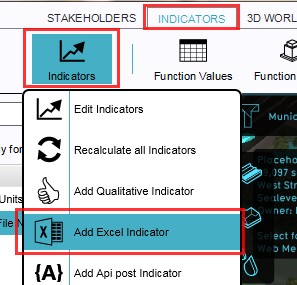
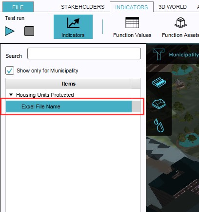
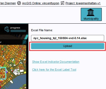
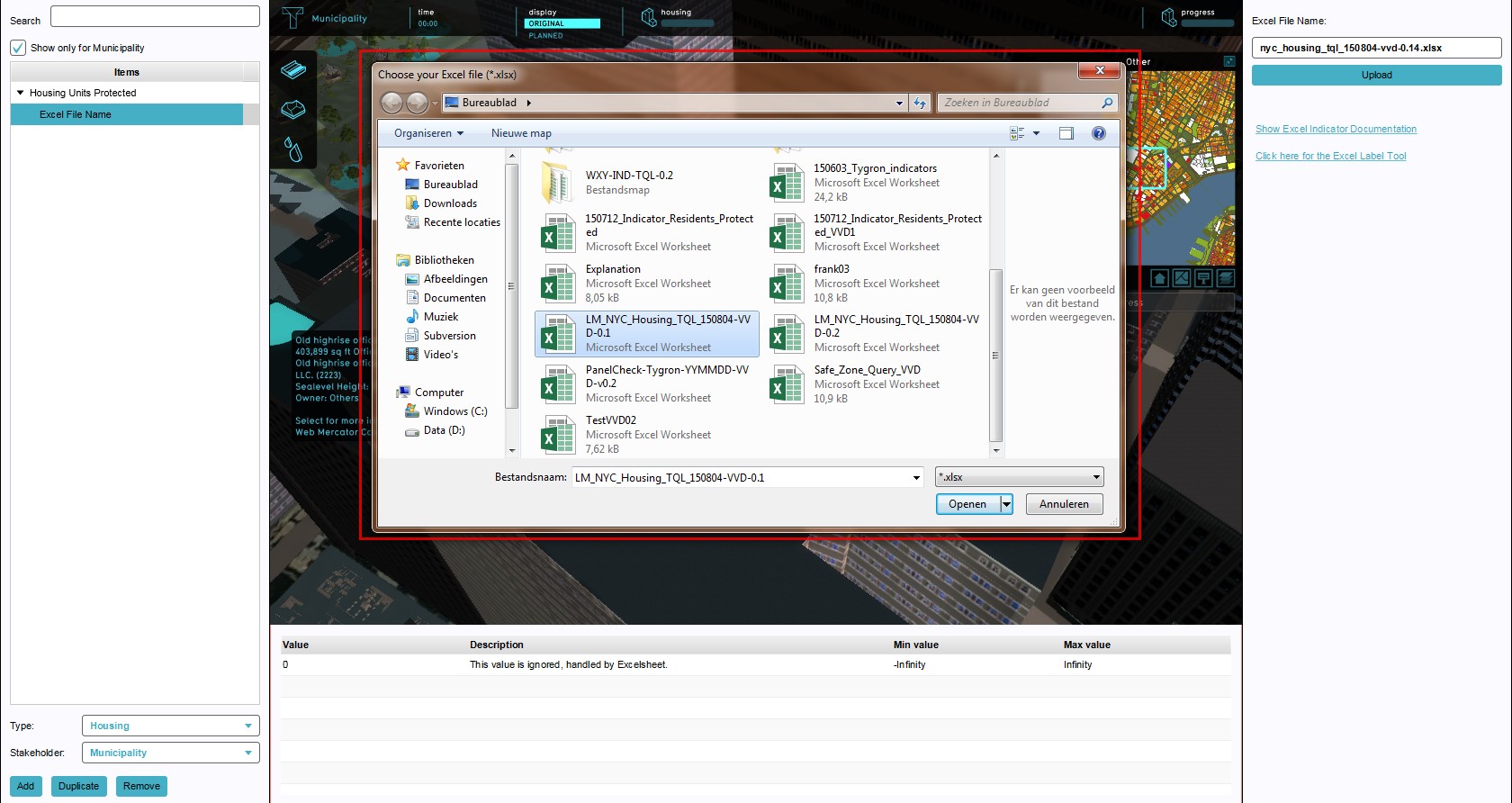
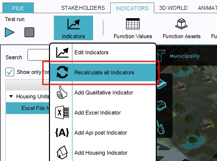
To upload an Excel xlsx-file for the Excel Indicator, have the file ready on an easy to remember location (desktop for instance), and add in the Editor an Excel indicator to the project. Select Excel File Name on the left panel and select the Upload button on the right panel. In the newly opened panel, select the file to upload and confirm. Now the file has been uploaded to the project, and the new indicator has appeared on the top bar. If there was already a previous version of the file present, please select the Recalculate Indicators option from the Indicators drop down menu, to ensure the newly uploaded spreadsheet has an actual impact on the project.
- Select Indicators > Add Excel Indicator
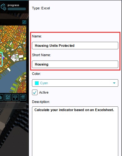
- Rename the newly added indicator in the 'Name' and Short Name' fields on the right panel
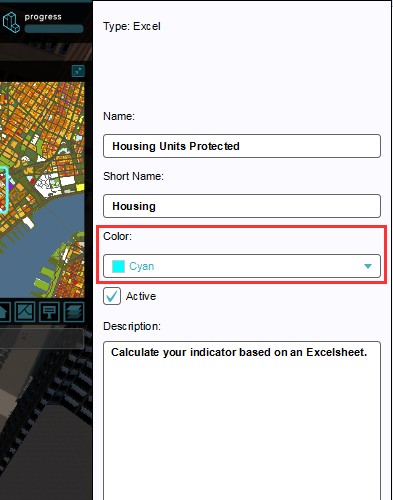
- Select the color to be used in the progression panel
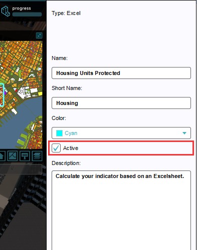
- Select to activate the indicator, if desired
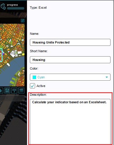
- Add a proper description
- Highlight 'Excel File Name' on the left panel panel
- Select the 'Upload' button
- Select the file to upload in the 'Choose your file' panel
- Select Indicators > recalculate Indicators
-
1. Select Indicators > Indicators > Add Excel Indicator
-
2. Enter new Name and Short Name
-
3. Change color of the indicator
-
4. Activate the indicator
-
5. Add a description
-
6. Highlight 'Excel File Name' on the left panel
-
7. Select the 'Upload' button
-
8. Select the file to upload in the 'Choose your file' panel
-
9. Recalculate the newly added Excel indicator
Summary (how to...)
- Below is a small summary describing a suggested workflow from a bird's eye perspective, without going deeper into details:
- Load the sample project Lower Manhattan in the editor.
- Create an empty xlsx workbook.
- Name one cell
EXPLANATION. - Create the
EXPLANATIONoutput format (HTML text string, HTML table) with%svariables. - Decide, based on the
EXPLANATION, which function categories are needed, and place them in one column. - Add consecutive columns that match the
EXPLANATION. - Create the
VARcolumns withROUND(UP)formulas andVAR_nname labels. - Create the
SCOREfield(s) as required by the type of project (Timeline/ Planning). - Optionally, test the spreadsheet by entering round values in query fields.
- Create a new Excel Indicator in the project and upload the Excel file to the project.
- Recalculate the indicators and verify if no errors are present.
Tips
- Divisions by zero can be solved as follows:
=C2/IF(D2,D2,1). In this example cells C2 and D2 contain number values. - Instead of using the VAR_# method for the explanation text, you can also use the concatenate function of excel:
CONCATENATE("<p>",A2, ": ", E2, " m2 and in Safe Zone: ", F2, " m2</p>")
- Starting with creating a table aids in setting up the Excel spreadsheet, by already thinking in advance about the lay out and formatting of the
EXPLANATION. - To quickly test the spreadsheet, without uploading it to the project, it is possible to enter some values in all the cells that contain queries as name. Other cells with formulas will change their content accordingly. By entering round values, for example 100, 1000, etc, calculations can easily be verified. Don't forget to save first and to revert back to the last saved version when done verifying!
- To display an actual percentage sign in the explanation, you need to place two percentage signs. I.e. : "50% of houses" should be written as "50%% of houses".
Extras
- As practice on these Excel indicators, try to create the following indicators for Lower Manhattan:
- Create an Excel indicator for protected floor sizes instead of for protected units of different categories.
- Create an Excel indicator for protected floor sizes of Industry, Offices and Commercial buildings.
- Create an Excel indicator for the amount of jobs being protected. Use for this the following constant values: Industry - 250sq ft/ job, Offices - 50sq ft/job and Commercial - 65sq ft/job.
How-to's
- How to configure a Query for an Excel Indicator
- How to create an Excel background calculation model
- How to implement an Excel Indicator
- How to manually adjust Indicators in Excel
- How to use the Query Tool to test queries from an Excel Indicator spreadsheet
